Chapter 6 Linear Models
6.1 Problem Setup
Both examples require some statistical model, but they are very different. The first is a causal inference problem: we want to design an intervention so that we need to recover the causal effect of temperature and pressure. The second is a prediction problem, a.k.a. a forecasting problem, in which we don’t care about the causal effects, we just want good predictions.
In this chapter we discuss the causal problem in Example 6.1. This means that when we assume a model, we assume it is the actual data generating process, i.e., we assume the sampling distribution is well specified. In the econometric literature, these are the structural equations. The second type of problems is discussed in the Supervised Learning Chapter 10.
Here are some more examples of the types of problems we are discussing.
Let’s present the linear model. We assume that a response7 variable is the sum of effects of some factors8. Denoting the response variable by \(y\), the factors by \(x=(x_1,\dots,x_p)\), and the effects by \(\beta:=(\beta_1,\dots,\beta_p)\) the linear model assumption implies that the expected response is the sum of the factors effects:
\[\begin{align} E[y]=x_1 \beta_1 + \dots + x_p \beta_p = \sum_{j=1}^p x_j \beta_j = x'\beta . \tag{6.1} \end{align}\] Clearly, there may be other factors that affect the the caps’ diameters. We thus introduce an error term9, denoted by \(\varepsilon\), to capture the effects of all unmodeled factors and measurement error10. The implied generative process of a sample of \(i=1,\dots,n\) observations it thus \[\begin{align} y_i = x_i'\beta + \varepsilon_i = \sum_j x_{i,j} \beta_j + \varepsilon_i , i=1,\dots,n . \tag{6.2} \end{align}\] or in matrix notation \[\begin{align} y = X \beta + \varepsilon . \tag{6.3} \end{align}\]
Let’s demonstrate Eq.(6.2). In our bottle-caps example [6.1], we may produce bottle caps at various temperatures. We design an experiment where we produce bottle-caps at varying temperatures. Let \(x_i\) be the temperature at which bottle-cap \(i\) was manufactured. Let \(y_i\) be its measured diameter. By the linear model assumption, the expected diameter varies linearly with the temperature: \(\mathbb{E}[y_i]=\beta_0 + x_i \beta_1\). This implies that \(\beta_1\) is the (expected) change in diameter due to a unit change in temperature.
There are many reasons linear models are very popular:
Before the computer age, these were pretty much the only models that could actually be computed11. The whole Analysis of Variance (ANOVA) literature is an instance of linear models, that relies on sums of squares, which do not require a computer to work with.
For purposes of prediction, where the actual data generating process is not of primary importance, they are popular because they simply work. Why is that? They are simple so that they do not require a lot of data to be computed. Put differently, they may be biased, but their variance is small enough to make them more accurate than other models.
For non continuous predictors, any functional relation can be cast as a linear model.
For the purpose of screening, where we only want to show the existence of an effect, and are less interested in the magnitude of that effect, a linear model is enough.
If the true generative relation is not linear, but smooth enough, then the linear function is a good approximation via Taylor’s theorem.
There are still two matters we have to attend: (i) How to estimate \(\beta\)? (ii) How to perform inference?
In the simplest linear models the estimation of \(\beta\) is done using the method of least squares. A linear model with least squares estimation is known as Ordinary Least Squares (OLS). The OLS problem:
\[\begin{align} \hat \beta:= argmin_\beta \{ \sum_i (y_i-x_i'\beta)^2 \}, \tag{6.4} \end{align}\] and in matrix notation \[\begin{align} \hat \beta:= argmin_\beta \{ \Vert y-X\beta \Vert^2_2 \}. \tag{6.5} \end{align}\]
Different software suits, and even different R packages, solve Eq.(6.4) in different ways so that we skip the details of how exactly it is solved. These are discussed in Chapters 17 and 18.
The last matter we need to attend is how to do inference on \(\hat \beta\). For that, we will need some assumptions on \(\varepsilon\). A typical set of assumptions is the following:
- Independence: we assume \(\varepsilon_i\) are independent of everything else. Think of them as the measurement error of an instrument: it is independent of the measured value and of previous measurements.
- Centered: we assume that \(E[\varepsilon]=0\), meaning there is no systematic error, sometimes it called The “Linearity assumption”.
- Normality: we will typically assume that \(\varepsilon \sim \mathcal{N}(0,\sigma^2)\), but we will later see that this is not really required.
We emphasize that these assumptions are only needed for inference on \(\hat \beta\) and not for the estimation itself, which is done by the purely algorithmic framework of OLS.
Given the above assumptions, we can apply some probability theory and linear algebra to get the distribution of the estimation error: \[\begin{align} \hat \beta - \beta \sim \mathcal{N}(0, (X'X)^{-1} \sigma^2). \tag{6.6} \end{align}\]
The reason I am not too strict about the normality assumption above, is that Eq.(6.6) is approximately correct even if \(\varepsilon\) is not normal, provided that there are many more observations than factors (\(n \gg p\)).
6.2 OLS Estimation in R
We are now ready to estimate some linear models with R.
We will use the whiteside data from the MASS package, recording the outside temperature and gas consumption, before and after an apartment’s insulation.
library(MASS) # load the package
library(data.table) # for some data manipulations
data(whiteside) # load the data
head(whiteside) # inspect the data
## Insul Temp Gas
## 1 Before -0.8 7.2
## 2 Before -0.7 6.9
## 3 Before 0.4 6.4
## 4 Before 2.5 6.0
## 5 Before 2.9 5.8
## 6 Before 3.2 5.8We do the OLS estimation on the pre-insulation data with lm function (acronym for Linear Model), possibly the most important function in R.
library(data.table)
whiteside <- data.table(whiteside)
lm.1 <- lm(Gas~Temp, data=whiteside[Insul=='Before']) # OLS estimation
Things to note:
- We used the tilde syntax
Gas~Temp, reading “gas as linear function of temperature”. - The
dataargument tells R where to look for the variables Gas and Temp. We usedInsul=='Before'to subset observations before the insulation. - The result is assigned to the object
lm.1.
Like any other language, spoken or programmable, there are many ways to say the same thing. Some more elegant than others…
lm.1 <- lm(y=Gas, x=Temp, data=whiteside[whiteside$Insul=='Before',])
lm.1 <- lm(y=whiteside[whiteside$Insul=='Before',]$Gas,x=whiteside[whiteside$Insul=='Before',]$Temp)
lm.1 <- whiteside[whiteside$Insul=='Before',] %>% lm(Gas~Temp, data=.)
The output is an object of class lm.
class(lm.1)## [1] "lm"Objects of class lm are very complicated.
They store a lot of information which may be used for inference, plotting, etc.
The str function, short for “structure”, shows us the various elements of the object.
str(lm.1)## List of 12
## $ coefficients : Named num [1:2] 6.854 -0.393
## ..- attr(*, "names")= chr [1:2] "(Intercept)" "Temp"
## $ residuals : Named num [1:26] 0.0316 -0.2291 -0.2965 0.1293 0.0866 ...
## ..- attr(*, "names")= chr [1:26] "1" "2" "3" "4" ...
## $ effects : Named num [1:26] -24.2203 -5.6485 -0.2541 0.1463 0.0988 ...
## ..- attr(*, "names")= chr [1:26] "(Intercept)" "Temp" "" "" ...
## $ rank : int 2
## $ fitted.values: Named num [1:26] 7.17 7.13 6.7 5.87 5.71 ...
## ..- attr(*, "names")= chr [1:26] "1" "2" "3" "4" ...
## $ assign : int [1:2] 0 1
## $ qr :List of 5
## ..$ qr : num [1:26, 1:2] -5.099 0.196 0.196 0.196 0.196 ...
## .. ..- attr(*, "dimnames")=List of 2
## .. .. ..$ : chr [1:26] "1" "2" "3" "4" ...
## .. .. ..$ : chr [1:2] "(Intercept)" "Temp"
## .. ..- attr(*, "assign")= int [1:2] 0 1
## ..$ qraux: num [1:2] 1.2 1.35
## ..$ pivot: int [1:2] 1 2
## ..$ tol : num 1e-07
## ..$ rank : int 2
## ..- attr(*, "class")= chr "qr"
## $ df.residual : int 24
## $ xlevels : Named list()
## $ call : language lm(formula = Gas ~ Temp, data = whiteside[Insul == "Before"])
## $ terms :Classes 'terms', 'formula' language Gas ~ Temp
## .. ..- attr(*, "variables")= language list(Gas, Temp)
## .. ..- attr(*, "factors")= int [1:2, 1] 0 1
## .. .. ..- attr(*, "dimnames")=List of 2
## .. .. .. ..$ : chr [1:2] "Gas" "Temp"
## .. .. .. ..$ : chr "Temp"
## .. ..- attr(*, "term.labels")= chr "Temp"
## .. ..- attr(*, "order")= int 1
## .. ..- attr(*, "intercept")= int 1
## .. ..- attr(*, "response")= int 1
## .. ..- attr(*, ".Environment")=<environment: R_GlobalEnv>
## .. ..- attr(*, "predvars")= language list(Gas, Temp)
## .. ..- attr(*, "dataClasses")= Named chr [1:2] "numeric" "numeric"
## .. .. ..- attr(*, "names")= chr [1:2] "Gas" "Temp"
## $ model :'data.frame': 26 obs. of 2 variables:
## ..$ Gas : num [1:26] 7.2 6.9 6.4 6 5.8 5.8 5.6 4.7 5.8 5.2 ...
## ..$ Temp: num [1:26] -0.8 -0.7 0.4 2.5 2.9 3.2 3.6 3.9 4.2 4.3 ...
## ..- attr(*, "terms")=Classes 'terms', 'formula' language Gas ~ Temp
## .. .. ..- attr(*, "variables")= language list(Gas, Temp)
## .. .. ..- attr(*, "factors")= int [1:2, 1] 0 1
## .. .. .. ..- attr(*, "dimnames")=List of 2
## .. .. .. .. ..$ : chr [1:2] "Gas" "Temp"
## .. .. .. .. ..$ : chr "Temp"
## .. .. ..- attr(*, "term.labels")= chr "Temp"
## .. .. ..- attr(*, "order")= int 1
## .. .. ..- attr(*, "intercept")= int 1
## .. .. ..- attr(*, "response")= int 1
## .. .. ..- attr(*, ".Environment")=<environment: R_GlobalEnv>
## .. .. ..- attr(*, "predvars")= language list(Gas, Temp)
## .. .. ..- attr(*, "dataClasses")= Named chr [1:2] "numeric" "numeric"
## .. .. .. ..- attr(*, "names")= chr [1:2] "Gas" "Temp"
## - attr(*, "class")= chr "lm"In RStudio it is particularly easy to extract objects. Just write your.object$ and press tab after the $ for auto-completion.
If we only want \(\hat \beta\), it can also be extracted with the coef function.
coef(lm.1)## (Intercept) Temp
## 6.8538277 -0.3932388Things to note:
R automatically adds an
(Intercept)term. This means we estimate \(Gas=\beta_0 + \beta_1 Temp + \varepsilon\) and not \(Gas=\beta_1 Temp + \varepsilon\). This makes sense because we are interested in the contribution of the temperature to the variability of the gas consumption about its mean, and not about zero.The effect of temperature, i.e., \(\hat \beta_1\), is -0.39. The negative sign means that the higher the temperature, the less gas is consumed. The magnitude of the coefficient means that for a unit increase in the outside temperature, the gas consumption decreases by 0.39 units.
We can use the predict function to make predictions, but we emphasize that if the purpose of the model is to make predictions, and not interpret coefficients, better skip to the Supervised Learning Chapter 10.
# Gas predictions (b0+b1*temperature) vs. actual Gas measurements, ideal slope should be 1.
plot(predict(lm.1)~whiteside[Insul=='Before',Gas])
# plots identity line (slope 1), lty=Line Type, 2 means dashed line.
abline(0,1, lty=2)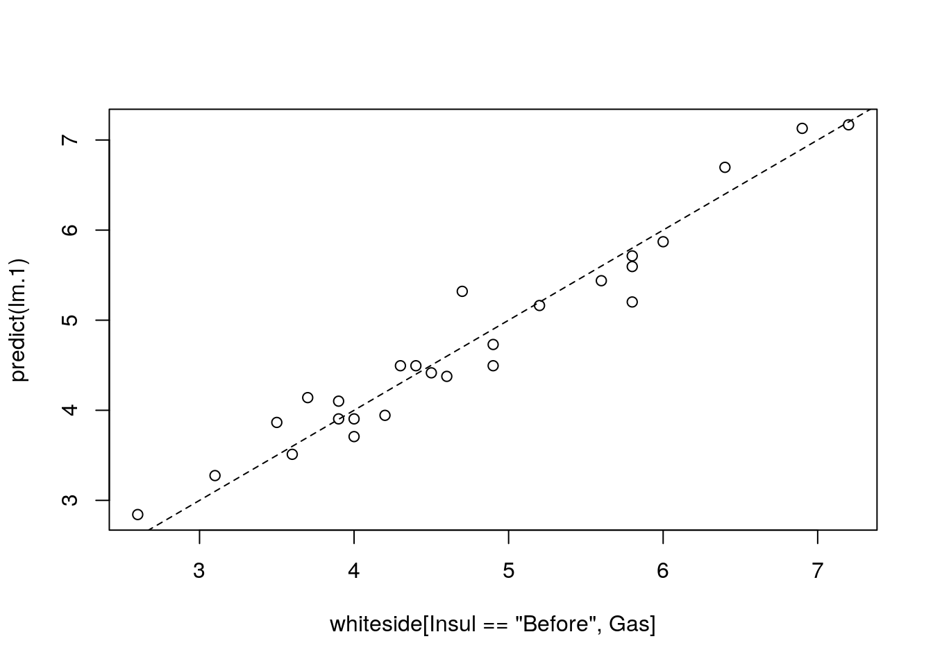
The model seems to fit the data nicely. A common measure of the goodness of fit is the coefficient of determination, more commonly known as the \(R^2\).
It can be easily computed
library(magrittr)
R2 <- function(y, y.hat){
  numerator <- (y-y.hat)^2 %>% sum
  denominator <- (y-mean(y))^2 %>% sum
  1-numerator/denominator
}
R2(y=whiteside[Insul=='Before',Gas], y.hat=predict(lm.1))
## [1] 0.9438081This is a nice result implying that about \(94\%\) of the variability in gas consumption can be attributed to changes in the outside temperature.
Obviously, R does provide the means to compute something as basic as \(R^2\), but I will let you find it for yourselves.
6.3 Inference
To perform inference on \(\hat \beta\), in order to test hypotheses and construct confidence intervals, we need to quantify the uncertainly in the reported \(\hat \beta\). This is exactly what Eq.(6.6) gives us.
Luckily, we don’t need to manipulate multivariate distributions manually, and everything we need is already implemented.
The most important function is summary which gives us an overview of the model’s fit.
We emphasize that fitting a model with lm is an assumption free algorithmic step.
Inference using summary is not assumption free, and requires the set of assumptions leading to Eq.(6.6).
summary(lm.1)##
## Call:
## lm(formula = Gas ~ Temp, data = whiteside[Insul == "Before"])
##
## Residuals:
## Min 1Q Median 3Q Max
## -0.62020 -0.19947 0.06068 0.16770 0.59778
##
## Coefficients:
## Estimate Std. Error t value Pr(>|t|)
## (Intercept) 6.85383 0.11842 57.88 <2e-16 ***
## Temp -0.39324 0.01959 -20.08 <2e-16 ***
## ---
## Signif. codes: 0 '***' 0.001 '**' 0.01 '*' 0.05 '.' 0.1 ' ' 1
##
## Residual standard error: 0.2813 on 24 degrees of freedom
## Multiple R-squared: 0.9438, Adjusted R-squared: 0.9415
## F-statistic: 403.1 on 1 and 24 DF, p-value: < 2.2e-16Things to note:
- The estimated \(\hat \beta\) is reported in the `Coefficients’ table, which has point estimates, standard errors, t-statistics, and the p-values of a two-sided hypothesis test for each coefficient \(H_{0,j}:\beta_j=0, j=1,\dots,p\).
- The \(R^2\) is reported at the bottom. The “Adjusted R-squared” is a variation that compensates for the model’s complexity.
- The original call to
lmis saved in theCallsection. - Some summary statistics of the residuals (\(y_i-\hat y_i\)) in the
Residualssection. - The “residuals standard error”12 is \(\sqrt{(n-p)^{-1} \sum_i (y_i-\hat y_i)^2}\). The denominator of this expression is the degrees of freedom, \(n-p\), which can be thought of as the hardness of the problem.
As the name suggests, summary is merely a summary. The full summary(lm.1) object is a monstrous object.
Its various elements can be queried using str(sumary(lm.1)).
Can we check the assumptions required for inference? Some. Let’s start with the linearity assumption. If we were wrong, and the data is not arranged about a linear line, the residuals will have some shape. We thus plot the residuals as a function of the predictor to diagnose shape.
# errors (epsilons) vs. temperature, should oscillate around zero.
plot(residuals(lm.1)~whiteside[Insul=='Before',Temp])
abline(0,0, lty=2)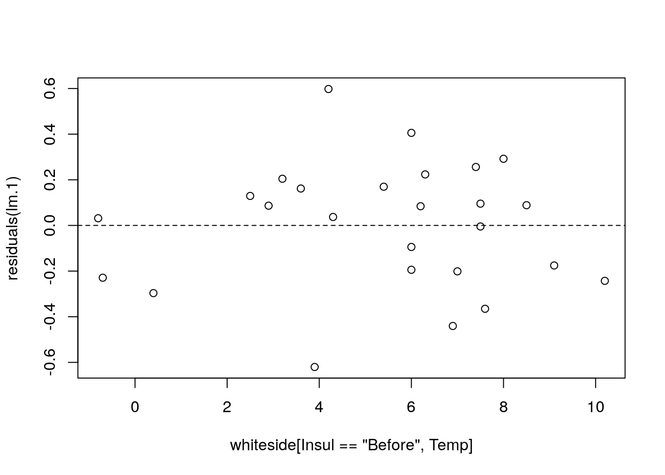
I can’t say I see any shape. Let’s fit a wrong model, just to see what “shape” means.
lm.1.1 <- lm(Gas~I(Temp^2), data=whiteside[Insul=='Before',])
plot(residuals(lm.1.1)~whiteside[Insul=='Before',Temp]); abline(0,0, lty=2)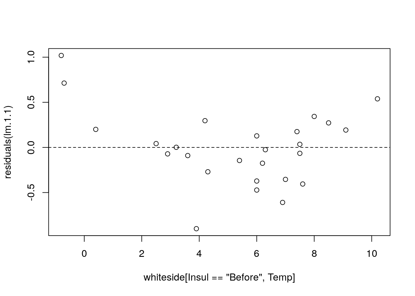
Things to note:
- We used
I(Temp^2)to specify the model \(Gas=\beta_0 + \beta_1 Temp^2+ \varepsilon\). - The residuals have a “belly”. Because they are not a cloud around the linear trend, and we have the wrong model.
To the next assumption.
We assumed \(\varepsilon_i\) are independent of everything else.
The residuals, \(y_i-\hat y_i\) can be thought of a sample of \(\varepsilon_i\).
When diagnosing the linearity assumption, we already saw their distribution does not vary with the \(x\)’s, Temp in our case.
They may be correlated with themselves; a positive departure from the model, may be followed by a series of positive departures etc.
Diagnosing these auto-correlations is a real art, which is not part of our course.
The last assumption we required is normality. As previously stated, if \(n \gg p\), this assumption can be relaxed. If \(n\) is in the order of \(p\), we need to verify this assumption. My favorite tool for this task is the qqplot. A qqplot compares the quantiles of the sample with the respective quantiles of the assumed distribution. If quantiles align along a line, the assumed distribution is OK. If quantiles depart from a line, then the assumed distribution does not fit the sample.
qqnorm(resid(lm.1))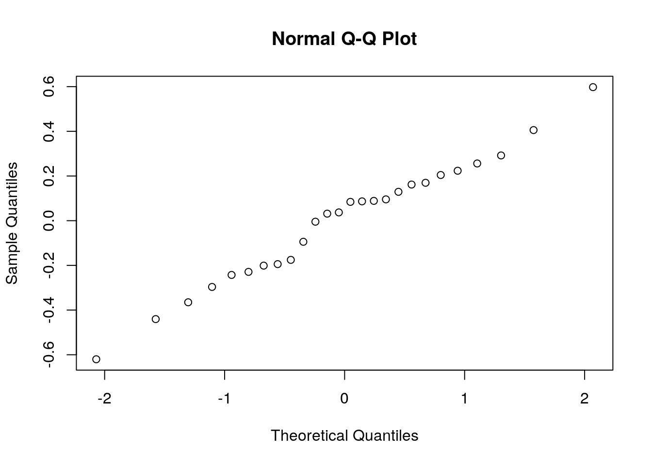
Things to note:
- The
qqnormfunction plots a qqplot against a normal distribution. For non-normal distributions tryqqplot. resid(lm.1)extracts the residuals from the linear model, i.e., the vector of \(y_i-x_i'\hat \beta\).
Judging from the figure, the normality assumption is quite plausible. Let’s try the same on a non-normal sample, namely a uniformly distributed sample, to see how that would look.
qqnorm(runif(100))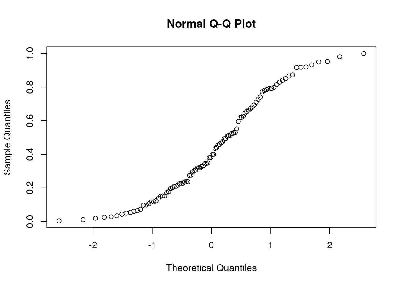
6.3.1 Testing a Hypothesis on a Single Coefficient
The first inferential test we consider is a hypothesis test on a single coefficient.
In our gas example, we may want to test that the temperature has no effect on the gas consumption.
The answer for that is given immediately by summary(lm.1)
summary.lm1 <- summary(lm.1)
coefs.lm1 <- summary.lm1$coefficients
coefs.lm1
## Estimate Std. Error t value Pr(>|t|)
## (Intercept) 6.8538277 0.11842341 57.87561 2.717533e-27
## Temp -0.3932388 0.01958601 -20.07754 1.640469e-16We see that the p-value for \(H_{0,1}: \beta_1=0\) against a two sided alternative is effectively 0 (row 2 column 4), so that \(\beta_1\) is unlikely to be \(0\) (the null hypothesis can be rejected).
6.3.2 Constructing a Confidence Interval on a Single Coefficient
Since the summary function gives us the standard errors of \(\hat \beta\), we can immediately compute \(\hat \beta_j \pm 2 \sqrt{Var[\hat \beta_j]}\) to get ourselves a (roughly) \(95\%\) confidence interval.
In our example the interval is
coefs.lm1[2,1] + c(-2,2) * coefs.lm1[2,2]## [1] -0.4324108 -0.3540668Things to note:
- The function
confint(lm.1)can calculate it. Sometimes it’s more simple to write 20 characters of code than finding a function that does it for us.
6.3.3 Multiple Regression
The swiss dataset encodes the fertility at each of Switzerland’s 47 French speaking provinces, along other socio-economic indicators. Let’s see if these are statistically related:
head(swiss)## Fertility Agriculture Examination Education Catholic
## Courtelary 80.2 17.0 15 12 9.96
## Delemont 83.1 45.1 6 9 84.84
## Franches-Mnt 92.5 39.7 5 5 93.40
## Moutier 85.8 36.5 12 7 33.77
## Neuveville 76.9 43.5 17 15 5.16
## Porrentruy 76.1 35.3 9 7 90.57
## Infant.Mortality
## Courtelary 22.2
## Delemont 22.2
## Franches-Mnt 20.2
## Moutier 20.3
## Neuveville 20.6
## Porrentruy 26.6lm.5 <- lm(data=swiss, Fertility~Agriculture+Examination+Education+Catholic+Infant.Mortality)
summary(lm.5)##
## Call:
## lm(formula = Fertility ~ Agriculture + Examination + Education +
## Catholic + Infant.Mortality, data = swiss)
##
## Residuals:
## Min 1Q Median 3Q Max
## -15.2743 -5.2617 0.5032 4.1198 15.3213
##
## Coefficients:
## Estimate Std. Error t value Pr(>|t|)
## (Intercept) 66.91518 10.70604 6.250 1.91e-07 ***
## Agriculture -0.17211 0.07030 -2.448 0.01873 *
## Examination -0.25801 0.25388 -1.016 0.31546
## Education -0.87094 0.18303 -4.758 2.43e-05 ***
## Catholic 0.10412 0.03526 2.953 0.00519 **
## Infant.Mortality 1.07705 0.38172 2.822 0.00734 **
## ---
## Signif. codes: 0 '***' 0.001 '**' 0.01 '*' 0.05 '.' 0.1 ' ' 1
##
## Residual standard error: 7.165 on 41 degrees of freedom
## Multiple R-squared: 0.7067, Adjusted R-squared: 0.671
## F-statistic: 19.76 on 5 and 41 DF, p-value: 5.594e-10Things to note:
- The
~syntax allows to specify various predictors separated by the+operator. - The summary of the model now reports the estimated effect, i.e., the regression coefficient, of each of the variables.
Clearly, naming each variable explicitly is a tedious task if there are many. The use of Fertility~. in the next example reads: “Fertility as a function of all other variables in the swiss data.frame”.
lm.5 <- lm(data=swiss, Fertility~.)
summary(lm.5)
##
## Call:
## lm(formula = Fertility ~ ., data = swiss)
##
## Residuals:
## Min 1Q Median 3Q Max
## -15.2743 -5.2617 0.5032 4.1198 15.3213
##
## Coefficients:
## Estimate Std. Error t value Pr(>|t|)
## (Intercept) 66.91518 10.70604 6.250 1.91e-07 ***
## Agriculture -0.17211 0.07030 -2.448 0.01873 *
## Examination -0.25801 0.25388 -1.016 0.31546
## Education -0.87094 0.18303 -4.758 2.43e-05 ***
## Catholic 0.10412 0.03526 2.953 0.00519 **
## Infant.Mortality 1.07705 0.38172 2.822 0.00734 **
## ---
## Signif. codes: 0 '***' 0.001 '**' 0.01 '*' 0.05 '.' 0.1 ' ' 1
##
## Residual standard error: 7.165 on 41 degrees of freedom
## Multiple R-squared: 0.7067, Adjusted R-squared: 0.671
## F-statistic: 19.76 on 5 and 41 DF, p-value: 5.594e-106.3.4 ANOVA (*)
Our next example13 contains a hypothetical sample of \(60\) participants who are divided into three stress reduction treatment groups (mental, physical, and medical) and three age groups groups. The stress reduction values are represented on a scale that ranges from 1 to 10. The values represent how effective the treatment programs were at reducing participant’s stress levels, with larger effects indicating higher effectiveness.
twoWay <- read.csv('data/dataset_anova_twoWay_comparisons.csv')
head(twoWay)
## Treatment Age StressReduction
## 1 mental young 10
## 2 mental young 9
## 3 mental young 8
## 4 mental mid 7
## 5 mental mid 6
## 6 mental mid 5How many observations per group?
table(twoWay$Treatment, twoWay$Age)##
## mid old young
## medical 3 3 3
## mental 3 3 3
## physical 3 3 3Since we have two factorial predictors, this multiple regression is nothing but a two way ANOVA. Let’s fit the model and inspect it.
lm.2 <- lm(StressReduction~.,data=twoWay)
summary(lm.2)
##
## Call:
## lm(formula = StressReduction ~ ., data = twoWay)
##
## Residuals:
## Min 1Q Median 3Q Max
## -1 -1 0 1 1
##
## Coefficients:
## Estimate Std. Error t value Pr(>|t|)
## (Intercept) 4.0000 0.3892 10.276 7.34e-10 ***
## Treatmentmental 2.0000 0.4264 4.690 0.000112 ***
## Treatmentphysical 1.0000 0.4264 2.345 0.028444 *
## Ageold -3.0000 0.4264 -7.036 4.65e-07 ***
## Ageyoung 3.0000 0.4264 7.036 4.65e-07 ***
## ---
## Signif. codes: 0 '***' 0.001 '**' 0.01 '*' 0.05 '.' 0.1 ' ' 1
##
## Residual standard error: 0.9045 on 22 degrees of freedom
## Multiple R-squared: 0.9091, Adjusted R-squared: 0.8926
## F-statistic: 55 on 4 and 22 DF, p-value: 3.855e-11Things to note:
The
StressReduction~.syntax is read as “Stress reduction as a function of everything else”.All the (main) effects and the intercept seem to be significant.
Mid age and medical treatment are missing, hence it is implied that they are the baseline, and this model accounts for the departure from this baseline.
The data has 2 factors, but the coefficients table has 4 predictors. This is because
lmnoticed thatTreatmentandAgeare factors. Each level of each factor is thus encoded as a different (dummy) variable. The numerical values of the factors are meaningless. Instead, R has constructed a dummy variable for each level of each factor. The names of the effect are a concatenation of the factor’s name, and its level. You can inspect these dummy variables with themodel.matrixcommand.
model.matrix(lm.2) %>% lattice::levelplot()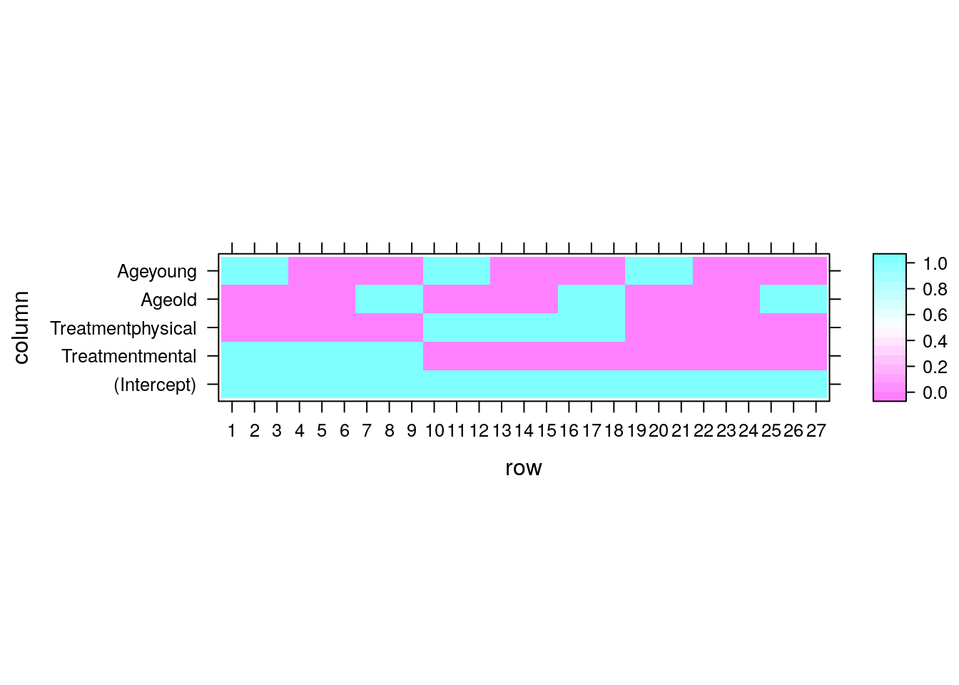 If you don’t want the default dummy coding, look at
 ?contrasts.
If you are more familiar with the ANOVA literature, or that you don’t want the effects of each level separately, but rather, the effect of all the levels of each factor, use the anova command.
anova(lm.2)## Analysis of Variance Table
##
## Response: StressReduction
## Df Sum Sq Mean Sq F value Pr(>F)
## Treatment 2 18 9.000 11 0.0004883 ***
## Age 2 162 81.000 99 1e-11 ***
## Residuals 22 18 0.818
## ---
## Signif. codes: 0 '***' 0.001 '**' 0.01 '*' 0.05 '.' 0.1 ' ' 1Things to note:
- The ANOVA table, unlike the
summaryfunction, tests if any of the levels of a factor has an effect, and not one level at a time. - The significance of each factor is computed using an F-test.
- The degrees of freedom, encoding the number of levels of a factor, is given in the
Dfcolumn. - The StressReduction seems to vary for different ages and treatments, since both factors are significant.
If you are extremely more comfortable with the ANOVA literature, you could have replaced the lm command with the aov command all along.
lm.2.2 <- aov(StressReduction~.,data=twoWay)
class(lm.2.2)
## [1] "aov" "lm"summary(lm.2.2)## Df Sum Sq Mean Sq F value Pr(>F)
## Treatment 2 18 9.00 11 0.000488 ***
## Age 2 162 81.00 99 1e-11 ***
## Residuals 22 18 0.82
## ---
## Signif. codes: 0 '***' 0.001 '**' 0.01 '*' 0.05 '.' 0.1 ' ' 1Things to note:
- The
lmfunction has been replaced with anaovfunction. - The output of
aovis anaovclass object, which extends thelmclass. - The summary of an
aovis not like the summary of anlmobject, but rather, like an ANOVA table.
As in any two-way ANOVA, we may want to ask if different age groups respond differently to different treatments. In the statistical parlance, this is called an interaction, or more precisely, an interaction of order 2.
lm.3 <- lm(StressReduction~Treatment+Age+Treatment:Age-1,data=twoWay)The syntax StressReduction~Treatment+Age+Treatment:Age-1 tells R to include main effects of Treatment, Age, and their interactions. The -1 removes the intercept.
Here are other ways to specify the same model.
lm.3 <- lm(StressReduction ~ Treatment * Age - 1,data=twoWay)
lm.3 <- lm(StressReduction~(.)^2 - 1,data=twoWay)
The syntax Treatment * Age means “main effects with second order interactions”.
The syntax (.)^2 means “everything with second order interactions”, this time we don’t have I() as in the temperature example because here we want the second order interaction and not the square of each variable.
Let’s inspect the model
summary(lm.3)##
## Call:
## lm(formula = StressReduction ~ Treatment + Age + Treatment:Age -
## 1, data = twoWay)
##
## Residuals:
## Min 1Q Median 3Q Max
## -1 -1 0 1 1
##
## Coefficients:
## Estimate Std. Error t value Pr(>|t|)
## Treatmentmedical 4.000e+00 5.774e-01 6.928 1.78e-06 ***
## Treatmentmental 6.000e+00 5.774e-01 10.392 4.92e-09 ***
## Treatmentphysical 5.000e+00 5.774e-01 8.660 7.78e-08 ***
## Ageold -3.000e+00 8.165e-01 -3.674 0.00174 **
## Ageyoung 3.000e+00 8.165e-01 3.674 0.00174 **
## Treatmentmental:Ageold 1.136e-16 1.155e+00 0.000 1.00000
## Treatmentphysical:Ageold 2.392e-16 1.155e+00 0.000 1.00000
## Treatmentmental:Ageyoung -1.037e-15 1.155e+00 0.000 1.00000
## Treatmentphysical:Ageyoung 2.564e-16 1.155e+00 0.000 1.00000
## ---
## Signif. codes: 0 '***' 0.001 '**' 0.01 '*' 0.05 '.' 0.1 ' ' 1
##
## Residual standard error: 1 on 18 degrees of freedom
## Multiple R-squared: 0.9794, Adjusted R-squared: 0.9691
## F-statistic: 95 on 9 and 18 DF, p-value: 2.556e-13Things to note:
- There are still \(5\) main effects, but also \(4\) interactions. This is because when allowing a different average response for every \(Treatment*Age\) combination, we are effectively estimating \(3*3=9\) cell means, even if they are not parametrized as cell means, but rather as main effect and interactions.
- The interactions do not seem to be significant.
- The assumptions required for inference are clearly not met in this example, which is there just to demonstrate R’s capabilities.
Asking if all the interactions are significant, is asking if the different age groups have the same response to different treatments.
Can we answer that based on the various interactions?
We might, but it is possible that no single interaction is significant, while the combination is.
To test for all the interactions together, we can simply check if the model without interactions is (significantly) better than a model with interactions. I.e., compare lm.2 to lm.3.
This is done with the anova command.
anova(lm.2,lm.3, test='F')## Analysis of Variance Table
##
## Model 1: StressReduction ~ Treatment + Age
## Model 2: StressReduction ~ Treatment + Age + Treatment:Age - 1
## Res.Df RSS Df Sum of Sq F Pr(>F)
## 1 22 18
## 2 18 18 4 7.1054e-15 0 1We see that lm.3 is not (significantly) better than lm.2, so that we can conclude that there are no interactions: different ages have the same response to different treatments.
6.3.5 Testing a Hypothesis on a Single Contrast (*)
Returning to the model without interactions, lm.2.
coef(summary(lm.2))## Estimate Std. Error t value Pr(>|t|)
## (Intercept) 4 0.3892495 10.276186 7.336391e-10
## Treatmentmental 2 0.4264014 4.690416 1.117774e-04
## Treatmentphysical 1 0.4264014 2.345208 2.844400e-02
## Ageold -3 0.4264014 -7.035624 4.647299e-07
## Ageyoung 3 0.4264014 7.035624 4.647299e-07We see that the effect of the various treatments is rather similar. It is possible that all treatments actually have the same effect. Comparing the effects of factor levels is called a contrast. Let’s test if the medical treatment, has in fact, the same effect as the physical treatment.
library(multcomp)
my.contrast <- matrix(c(-1,0,1,0,0), nrow =  1)
lm.4 <- glht(lm.2, linfct=my.contrast)
summary(lm.4)
##
## Simultaneous Tests for General Linear Hypotheses
##
## Fit: lm(formula = StressReduction ~ ., data = twoWay)
##
## Linear Hypotheses:
## Estimate Std. Error t value Pr(>|t|)
## 1 == 0 -3.0000 0.7177 -4.18 0.000389 ***
## ---
## Signif. codes: 0 '***' 0.001 '**' 0.01 '*' 0.05 '.' 0.1 ' ' 1
## (Adjusted p values reported -- single-step method)Things to note:
- A contrast is a linear function of the coefficients. In our example \(H_0:\beta_1-\beta_3=0\), which justifies the construction of
my.contrast. - We used the
glhtfunction (generalized linear hypothesis test) from the package multcomp. - The contrast is significant, i.e., the effect of a medical treatment, is different than that of a physical treatment.
6.4 Extra Diagnostics
6.4.1 Diagnosing Heteroskedasticity
Textbook assumptions for inference on \(\hat \beta_{OLS}\) include the homoskedasticiy assumption, i.e., \(Var[\varepsilon]\) is fixed and independent of everyhting. This comes from viewing \(\varepsilon\) as a measurement error. It may not be the case when viewing \(\varepsilon\) as “all other effect not included in the model”. In technical terms, homoskedastocity implies that \(Var[\varepsilon]\) is a scaled identity matrix. Heteroskedasticity means that \(Var[\varepsilon]\) is a diagonal matrix. Because a scaled identify matrix implies that the quantiles of a multivariate Gaussian are spheres, testing for heteroskedasticity is also known as a Sphericity Test.
Can we verify homoskedasticity, and do we need it?
To verify homoskedasticity we only need to look at the residuals of a model. If they seem to have the same variability for all \(x\) we are clear. If \(x\) is multivariate, and we cannot visualise residuals, \(y_i-\hat y_i\) as a function of \(x\), then visualising it as a function of \(\hat y_i\) is also good.
Another way of dealing with heteroskedasticity is by estimating variances for groups of observations separately. This is the Cluster Robust Standard Errors discussed in 8.4.1.
Can use perform a test to infer homoskedasticity? In the frequentist hypotesis testing framework we can only reject homoskedasticity, not accept it. In the Bayesian hypotesis testing framework we can indeed infer homoskedasticity, but one would have to defend his/her priors.
For some tests that detect heteroskedasticity see the olsrr package. For an econometric flavored approach to the problem, see the plm package, and its excellent vignette.
6.4.2 Diagnosing Multicolinearity
When designing an experiment (e.g. RCTs) we will assure treatments are “balanced”, so that one effect estimates are not correlated. This is not always possible, especially not in observational studies. If various variables capture the same effect, the certainty in the effect will “spread” over these variables. Formally: the standard errros of effect estimates will increase. Perhaps more importantly- causal inference with correlated predictors is very hard to interpret, because changes in outcome may be attibuted to any on of the (correlated) predictors.
We will eschew the complicated philosophical implication of causal infernece with correlated predictors, and merely refer the reader to the package olsrr for some popular tools to diagnose multicolinearity.
6.5 Bibliographic Notes
Like any other topic in this book, you can consult Venables and Ripley (2013) for more on linear models. For the theory of linear models, I like Greene (2003).
6.6 Practice Yourself
- Inspect women’s heights and weights with
?women.- What is the change in weight per unit change in height? Use the
lmfunction. - Is the relation of height on weight significant? Use
summary. - Plot the residuals of the linear model with
plotandresid. - Plot the predictions of the model using
abline. - Inspect the normality of residuals using
qqnorm. - Inspect the design matrix using
model.matrix.
- What is the change in weight per unit change in height? Use the
- Write a function that takes an
lmclass object, and returns the confidence interval on the first coefficient. Apply it on the height and weight data. Use the
ANOVAfunction to test the significance of the effect of height.- Read about the “mtcars” dataset using
? mtcars. Inspect the dependency of the fuel consumption (mpg) in the weight (wt) and the 1/4 mile time (qsec).- Make a pairs scatter plot with
plot(mtcars[,c("mpg","wt","qsec")])Does the connection look linear? - Fit a multiple linear regression with
lm. Call itmodel1. - Try to add the transmission (am) as independent variable. Let R know this is a categorical variable with
factor(am). Call itmodel2. - Compare the “Adjusted R-squared” measure of the two models (we can’t use the regular R2 to compare two models with a different number of variables).
- Do the coefficients significant?
- Inspect the normality of residuals and the linearity assumptions.
- Now Inspect the hypothesis that the effect of weight is different between the transmission types with adding interaction to the model
wt*factor(am). - According to this model, what is the addition of one unit of weight in a manual transmission to the fuel consumption (-2.973-4.141=-7.11)?
- Make a pairs scatter plot with
References
Friedman, Jerome, Trevor Hastie, and Robert Tibshirani. 2001. The Elements of Statistical Learning. Vol. 1. Springer series in statistics Springer, Berlin.
Greene, William H. 2003. Econometric Analysis. Pearson Education India.
Venables, William N, and Brian D Ripley. 2013. Modern Applied Statistics with S-Plus. Springer Science & Business Media.
The “response” is also known as the “dependent” variable in the statistical literature, or the “labels” in the machine learning literature.↩
The “factors” are also known as the “independent variable”, or “the design”, in the statistical literature, and the “features”, or “attributes” in the machine learning literature.↩
The “error term” is also known as the “noise”, or the “common causes of variability”.↩
You may philosophize if the measurement error is a mere instance of unmodeled factors or not, but this has no real implication for our purposes.↩
By “computed” we mean what statisticians call “fitted”, or “estimated”, and computer scientists call “learned”.↩
Sometimes known as the Root Mean Squared Error (RMSE).↩
The example is taken from http://rtutorialseries.blogspot.co.il/2011/02/r-tutorial-series-two-way-anova-with.html↩