Chapter 9 Multivariate Data Analysis
The term “multivariate data analysis” is so broad and so overloaded, that we start by clarifying what is discussed and what is not discussed in this chapter. Broadly speaking, we will discuss statistical inference, and leave more “exploratory flavored” matters like clustering, and visualization, to the Unsupervised Learning Chapter 11.
We start with an example.
Formally, let \(y\) be single (random) measurement of a \(p\)-variate random vector. Denote \(\mu:=E[y]\). Here is the set of problems we will discuss, in order of their statistical difficulty.
Signal Detection: a.k.a. multivariate test, or global test, or omnibus test. Where we test whether \(\mu\) differs than some \(\mu_0\).
Signal Counting: a.k.a. prevalence estimation, or \(\pi_0\) estimation. Where we count the number of entries in \(\mu\) that differ from \(\mu_0\).
Signal Identification: a.k.a. selection, or multiple testing. Where we infer which of the entries in \(\mu\) differ from \(\mu_0\). In the ANOVA literature, this is known as a post-hoc analysis, which follows an omnibus test.
Estimation: Estimating the magnitudes of entries in \(\mu\), and their departure from \(\mu_0\). If estimation follows a signal detection or signal identification stage, this is known as selective estimation.
9.1 Signal Detection
Signal detection deals with the detection of the departure of \(\mu\) from some \(\mu_0\), and especially, \(\mu_0=0\). This problem can be thought of as the multivariate counterpart of the univariate hypothesis t-test.
9.1.1 Hotelling’s T2 Test
The most fundamental approach to signal detection is a mere generalization of the t-test, known as Hotelling’s \(T^2\) test.
Recall the univariate t-statistic of a data vector \(x\) of length \(n\): \[\begin{align} t^2(x):= \frac{(\bar{x}-\mu_0)^2}{Var[\bar{x}]}= (\bar{x}-\mu_0)Var[\bar{x}]^{-1}(\bar{x}-\mu_0), \tag{9.1} \end{align}\] where \(Var[\bar{x}]=S^2(x)/n\), and \(S^2(x)\) is the unbiased variance estimator \(S^2(x):=(n-1)^{-1}\sum (x_i-\bar x)^2\).
Generalizing Eq(9.1) to the multivariate case: \(\mu_0\) is a \(p\)-vector, \(\bar x\) is a \(p\)-vector, and \(Var[\bar x]\) is a \(p \times p\) matrix of the covariance between the \(p\) coordinated of \(\bar x\). When operating with vectors, the squaring becomes a quadratic form, and the division becomes a matrix inverse. We thus have \[\begin{align} T^2(x):= (\bar{x}-\mu_0)' Var[\bar{x}]^{-1} (\bar{x}-\mu_0), \tag{9.2} \end{align}\] which is the definition of Hotelling’s \(T^2\) one-sample test statistic. We typically denote the covariance between coordinates in \(x\) with \(\hat \Sigma(x)\), so that \(\widehat \Sigma_{k,l}:=\widehat {Cov}[x_k,x_l]=(n-1)^{-1} \sum (x_{k,i}-\bar x_k)(x_{l,i}-\bar x_l)\). Using the \(\Sigma\) notation, Eq.(9.2) becomes \[\begin{align} T^2(x):= n (\bar{x}-\mu_0)' \hat \Sigma(x)^{-1} (\bar{x}-\mu_0), \end{align}\] which is the standard notation of Hotelling’s test statistic.
For inference, we need the null distribution of Hotelling’s test statistic. For this we introduce some vocabulary17:
- Low Dimension: We call a problem low dimensional if \(n \gg p\), i.e. \(p/n \approx 0\). This means there are many observations per estimated parameter.
- High Dimension: We call a problem high dimensional if \(p/n \to c\), where \(c\in (0,1)\). This means there are more observations than parameters, but not many.
- Very High Dimension: We call a problem very high dimensional if \(p/n \to c\), where \(1<c<\infty\). This means there are less observations than parameters.
Hotelling’s \(T^2\) test can only be used in the low dimensional regime. For some intuition on this statement, think of taking \(n=20\) measurements of \(p=100\) physiological variables. We seemingly have \(20\) observations, but there are \(100\) unknown quantities in \(\mu\). Say you decide that \(\mu\) differs from \(\mu_0\) based on the coordinate with maximal difference between your data and \(\mu_0\). Do you know how much variability to expect of this maximum? Try comparing your intuition with a quick simulation. Did the variabilty of the maximum surprise you? Hotelling’s \(T^2\) is not the same as the maxiumum, but the same intuition applies. This criticism is formalized in Bai and Saranadasa (1996). In modern applications, Hotelling’s \(T^2\) is rarely recommended. Luckily, many modern alternatives are available. See J. Rosenblatt, Gilron, and Mukamel (2016) for a review.
9.1.2 Various Types of Signal to Detect
In the previous, we assumed that the signal is a departure of \(\mu\) from some \(\mu_0\). For vactor-valued data \(y\), that is distributed \(\mathcal F\), we may define “signal” as any departure from some \(\mathcal F_0\). This is the multivaraite counterpart of goodness-of-fit (GOF) tests.
Even when restricting “signal” to departures of \(\mu\) from \(\mu_0\), “signal” may come in various forms:
- Dense Signal: when the departure is in a large number of coordinates of \(\mu\).
- Sparse Signal: when the departure is in a small number of coordinates of \(\mu\).
Process control in a manufactoring plant, for instance, is consistent with a dense signal: if a manufacturing process has failed, we expect a change in many measurements (i.e. coordinates of \(\mu\)). Detection of activation in brain imaging is consistent with a dense signal: if a region encodes cognitive function, we expect a change in many brain locations (i.e. coordinates of \(\mu\).) Detection of disease encodig regions in the genome is consistent with a sparse signal: if susceptibility of disease is genetic, only a small subset of locations in the genome will encode it.
Hotelling’s \(T^2\) statistic is best for dense signal. The next test, is a simple (and forgotten) test best with sparse signal.
9.1.3 Simes’ Test
Hotelling’s \(T^2\) statistic has currently two limitations: It is designed for dense signals, and it requires estimating the covariance, which is a very difficult problem.
An algorithm, that is sensitive to sparse signal and allows statistically valid detection under a wide range of covariances (even if we don’t know the covariance) is known as Simes’ Test. The statistic is defined vie the following algorithm:
- Compute \(p\) variable-wise p-values: \(p_1,\dots,p_j\).
- Denote \(p_{(1)},\dots,p_{(j)}\) the sorted p-values.
- Simes’ statistic is \(p_{Simes}:=min_j\{p_{(j)} \times p/j\}\).
- Reject the “no signal” null hypothesis at significance \(\alpha\) if \(p_{Simes}<\alpha\).
9.1.4 Signal Detection with R
We start with simulating some data with no signal. We will convince ourselves that Hotelling’s and Simes’ tests detect nothing, when nothing is present. We will then generate new data, after injecting some signal, i.e., making \(\mu\) depart from \(\mu_0=0\). We then convince ourselves, that both Hotelling’s and Simes’ tests, are indeed capable of detecting signal, when present.
Generating null data:
library(mvtnorm)
n <- 100 # observations
p <- 18 # parameter dimension
mu <- rep(0,p) # no signal: mu=0
x <- rmvnorm(n = n, mean = mu)
dim(x)
## [1] 100 18lattice::levelplot(x) # just looking at white noise.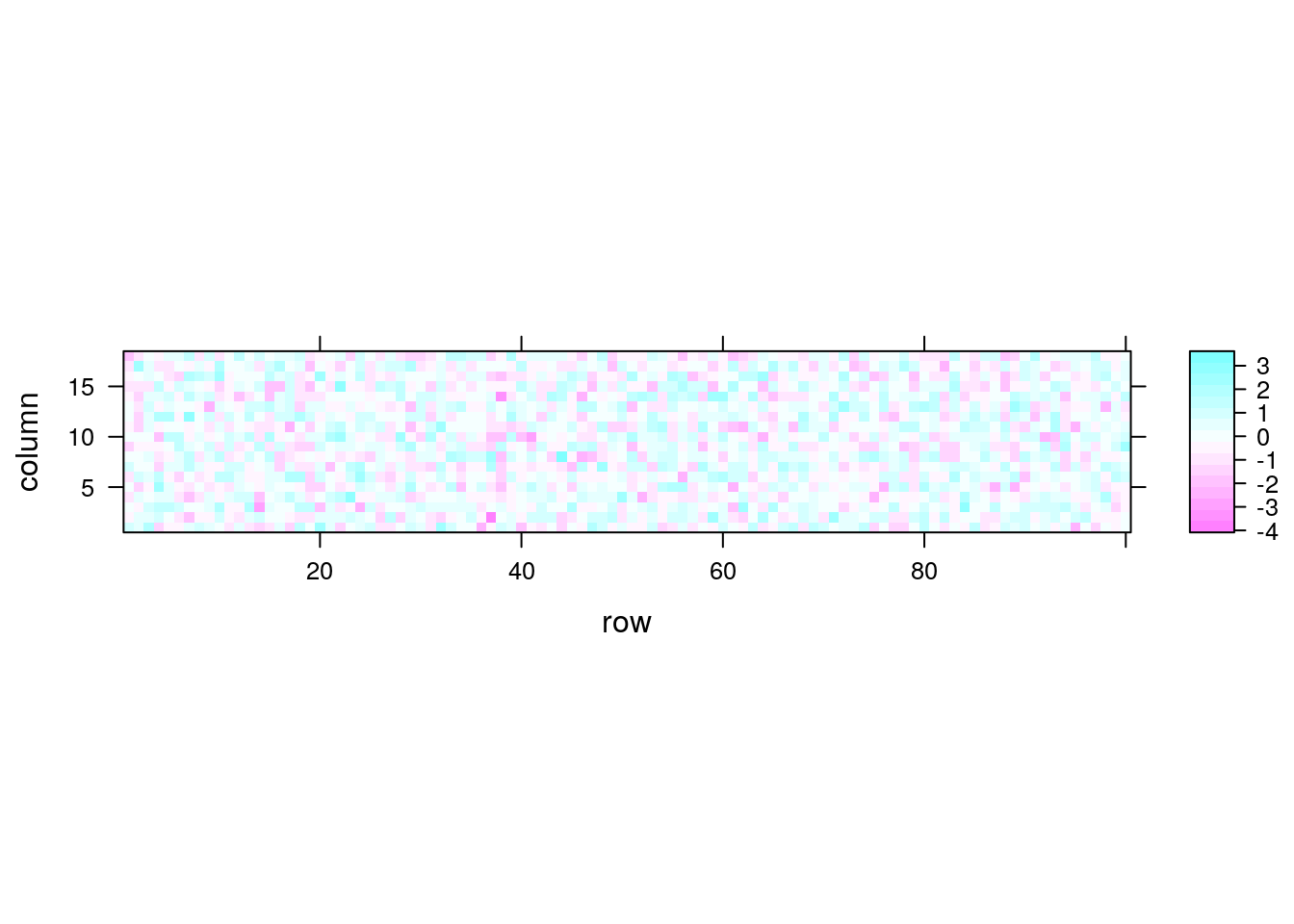
Now making our own Hotelling one-sample \(T^2\) test using Eq.((9.2)).
hotellingOneSample <- function(x, mu0=rep(0,ncol(x))){
  n <- nrow(x)
  p <- ncol(x)
  stopifnot(n > 5* p)
  bar.x <- colMeans(x)
  Sigma <- var(x)
  Sigma.inv <- solve(Sigma)
  T2 <- n * (bar.x-mu0) %*% Sigma.inv %*% (bar.x-mu0)
  p.value <- pchisq(q = T2, df = p, lower.tail = FALSE)
  return(list(statistic=T2, pvalue=p.value))
}
hotellingOneSample(x)
## $statistic
## [,1]
## [1,] 17.94698
##
## $pvalue
## [,1]
## [1,] 0.4591507Things to note:
stopifnot(n > 5 * p)is a little verification to check that the problem is indeed low dimensional. Otherwise, the \(\chi^2\) approximation cannot be trusted.solvereturns a matrix inverse.%*%is the matrix product operator (see alsocrossprod()).- A function may return only a single object, so we wrap the statistic and its p-value in a
listobject.
Just for verification, we compare our home made Hotelling’s test, to the implementation in the rrcov package. The statistic is clearly OK, but our \(\chi^2\) approximation of the distribution leaves room to desire. Personally, I would never trust a Hotelling test if \(n\) is not much greater than \(p\), in which case I would use a high-dimensional adaptation (see Bibliography).
rrcov::T2.test(x)##
## One-sample Hotelling test
##
## data: x
## T2 = 17.94698, F = 0.82584, df1 = 18, df2 = 82, p-value = 0.6653
## alternative hypothesis: true mean vector is not equal to (0, 0, 0, 0, 0, 0, 0, 0, 0, 0, 0, 0, 0, 0, 0, 0, 0, 0)'
##
## sample estimates:
## [,1] [,2] [,3] [,4] [,5]
## mean x-vector -0.002990837 0.06118945 0.2153931 -0.0487018 -0.06665223
## [,6] [,7] [,8] [,9] [,10]
## mean x-vector 0.1297716 0.04790746 0.08328193 -0.08511783 0.02627395
## [,11] [,12] [,13] [,14] [,15]
## mean x-vector -0.09120245 0.1603455 0.1298308 0.08406651 -0.0559366
## [,16] [,17] [,18]
## mean x-vector 0.03307495 -0.04411712 -0.1185427Let’s do the same with Simes’:
Simes <- function(x){
  p.vals <- apply(x, 2, function(z) t.test(z)$p.value) # Compute variable-wise pvalues
  p <- ncol(x)
  p.Simes <- p * min(sort(p.vals)/seq_along(p.vals)) # Compute the Simes statistic
  return(c(pvalue=p.Simes))
}
Simes(x)
## pvalue
## 0.4937222And now we verify that both tests can indeed detect signal when present. Are p-values small enough to reject the “no signal” null hypothesis?
mu <- rep(x = 10/p,times=p) # inject signal
x <- rmvnorm(n = n, mean = mu)
hotellingOneSample(x)
## $statistic
## [,1]
## [1,] 804.2087
##
## $pvalue
## [,1]
## [1,] 4.038321e-159Simes(x)## pvalue
## 2.76579e-10… yes. All p-values are very small, so that all statistics can detect the non-null distribution.
9.2 Signal Counting
There are many ways to approach the signal counting problem. For the purposes of this book, however, we will not discuss them directly, and solve the signal counting problem as a signal identification problem: if we know where \(\mu\) departs from \(\mu_0\), we only need to count coordinates to solve the signal counting problem.
9.3 Signal Identification
The problem of signal identification is also known as selective testing, or more commonly as multiple testing.
In the ANOVA literature, an identification stage will typically follow a detection stage. These are known as the omnibus F test, and post-hoc tests, respectively. In the multiple testing literature there will typically be no preliminary detection stage. It is typically assumed that signal is present, and the only question is “where?”
The first question when approaching a multiple testing problem is “what is an error”? Is an error declaring a coordinate in \(\mu\) to be different than \(\mu_0\) when it is actually not? Is an error an overly high proportion of falsely identified coordinates? The former is known as the family wise error rate (FWER), and the latter as the false discovery rate (FDR).
9.3.1 Signal Identification in R
One (of many) ways to do signal identification involves the stats::p.adjust function.
The function takes as inputs a \(p\)-vector of the variable-wise p-values.
Why do we start with variable-wise p-values, and not the full data set?
- Because we want to make inference variable-wise, so it is natural to start with variable-wise statistics.
- Because we want to avoid dealing with covariances if possible. Computing variable-wise p-values does not require estimating covariances.
- So that the identification problem is decoupled from the variable-wise inference problem, and may be applied much more generally than in the setup we presented.
We start be generating some high-dimensional multivariate data and computing the coordinate-wise (i.e. hypothesis-wise) p-value.
library(mvtnorm)
n <- 1e1
p <- 1e2
mu <- rep(0,p)
x <- rmvnorm(n = n, mean = mu)
dim(x)
## [1] 10 100lattice::levelplot(x)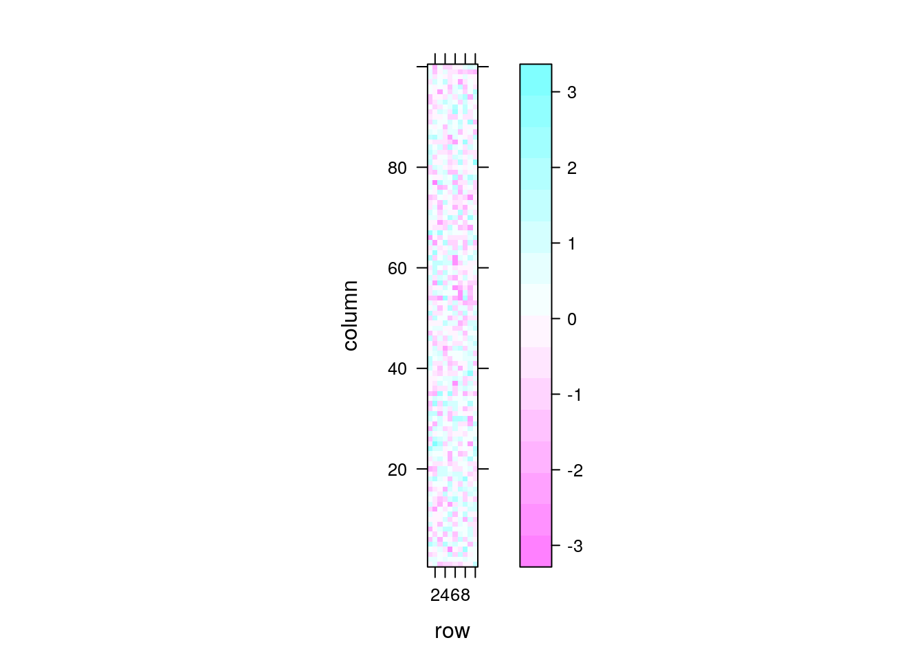
We now compute the pvalues of each coordinate. We use a coordinate-wise t-test. Why a t-test? Because for the purpose of demonstration we want a simple test. In reality, you may use any test that returns valid p-values.
t.pval <- function(y) t.test(y)$p.value
p.values <- apply(X = x, MARGIN = 2, FUN = t.pval)
plot(p.values, type='h')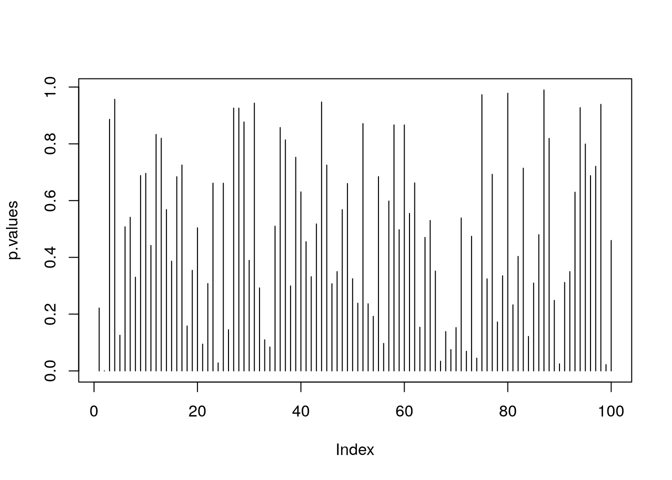
Things to note:
t.pvalis a function that merely returns the p-value of a t.test.- We used the
applyfunction to apply the same function to each column ofx. MARGIN=2tellsapplyto compute over columns and not rows.- The output,
p.values, is a vector of 100 p-values.
We are now ready to do the identification, i.e., find which coordinate of \(\mu\) is different than \(\mu_0=0\). The workflow for identification has the same structure, regardless of the desired error guarantees:
- Compute an
adjusted p-value. - Compare the adjusted p-value to the desired error level.
If we want \(FWER \leq 0.05\), meaning that we allow a \(5\%\) probability of making any mistake, we will use the method="holm" argument of p.adjust.
alpha <- 0.05
p.values.holm <- p.adjust(p.values, method = 'holm' )
which(p.values.holm < alpha)
## integer(0)If we want \(FDR \leq 0.05\), meaning that we allow the proportion of false discoveries to be no larger than \(5\%\), we use the method="BH" argument of p.adjust.
alpha <- 0.05
p.values.BH <- p.adjust(p.values, method = 'BH' )
which(p.values.BH < alpha)
## integer(0)We now inject some strong signal in \(\mu\) just to see that the process works. We will artificially inject signal in the first 10 coordinates.
mu[1:10] <- 2 # inject signal in first 10 variables
x <- rmvnorm(n = n, mean = mu) # generate data
p.values <- apply(X = x, MARGIN = 2, FUN = t.pval)
p.values.BH <- p.adjust(p.values, method = 'BH' )
which(p.values.BH < alpha)
## [1] 1 2 3 4 5 6 7 8 9 10Indeed- we are now able to detect that the first coordinates carry signal, because their respective coordinate-wise null hypotheses have been rejected.
9.4 Signal Estimation (*)
The estimation of the elements of \(\mu\) is a seemingly straightforward task. This is not the case, however, if we estimate only the elements that were selected because they were significant (or any other data-dependent criterion). Clearly, estimating only significant entries will introduce a bias in the estimation. In the statistical literature, this is known as selection bias. Selection bias also occurs when you perform inference on regression coefficients after some model selection, say, with a lasso, or a forward search18.
Selective inference is a complicated and active research topic so we will not offer any off-the-shelf solution to the matter. The curious reader is invited to read Rosenblatt and Benjamini (2014), Javanmard and Montanari (2014), or Will Fithian’s PhD thesis (Fithian 2015) for more on the topic.
9.5 Bibliographic Notes
For a general introduction to multivariate data analysis see Anderson-Cook (2004). For an R oriented introduction, see Everitt and Hothorn (2011). For more on the difficulties with high dimensional problems, see Bai and Saranadasa (1996). For some cutting edge solutions for testing in high-dimension, see J. Rosenblatt, Gilron, and Mukamel (2016) and references therein. Simes’ test is not very well known. It is introduced in Simes (1986), and proven to control the type I error of detection under a PRDS type of dependence in Benjamini and Yekutieli (2001). For more on multiple testing, and signal identification, see Efron (2012). For more on the choice of your error rate see Rosenblatt (2013). For an excellent review on graphical models see Kalisch and Bühlmann (2014). Everything you need on graphical models, Bayesian belief networks, and structure learning in R, is collected in the Task View.
9.6 Practice Yourself
Generate multivariate data with:
set.seed(3) mu<-rexp(50,6) multi<- rmvnorm(n = 100, mean = mu)- Use Hotelling’s test to determine if \(\mu\) equals \(\mu_0=0\). Can you detect the signal?
- Perform t.test on each variable and extract the p-value. Try to identify visually the variables which depart from \(\mu_0\).
- Use
p.adjustto identify in which variables there are any departures from \(\mu_0=0\). Allow 5% probability of making any false identification. - Use
p.adjustto identify in which variables there are any departures from \(\mu_0=0\). Allow a 5% proportion of errors within identifications.
- Generate multivariate data from two groups:
rmvnorm(n = 100, mean = rep(0,10))for the first, andrmvnorm(n = 100, mean = rep(0.1,10))for the second.- Do we agree the groups differ?
- Implement the two-group Hotelling test described in Wikipedia: (https://en.wikipedia.org/wiki/Hotelling%27s_T-squared_distribution#Two-sample_statistic).
- Verify that you are able to detect that the groups differ.
- Perform a two-group t-test on each coordinate. On which coordinates can you detect signal while controlling the FWER? On which while controlling the FDR? Use
p.adjust.
Return to the previous problem, but set
n=9. Verify that you cannot compute your Hotelling statistic.
References
Anderson-Cook, Christine M. 2004. “An Introduction to Multivariate Statistical Analysis.” Journal of the American Statistical Association 99 (467). American Statistical Association: 907–9.
Bai, Zhidong, and Hewa Saranadasa. 1996. “Effect of High Dimension: By an Example of a Two Sample Problem.” Statistica Sinica. JSTOR, 311–29.
Benjamini, Yoav, and Daniel Yekutieli. 2001. “The Control of the False Discovery Rate in Multiple Testing Under Dependency.” Annals of Statistics. JSTOR, 1165–88.
Efron, Bradley. 2012. Large-Scale Inference: Empirical Bayes Methods for Estimation, Testing, and Prediction. Vol. 1. Cambridge University Press.
Everitt, Brian, and Torsten Hothorn. 2011. An Introduction to Applied Multivariate Analysis with R. Springer Science & Business Media.
Fithian, William. 2015. “Topics in Adaptive Inference.” PhD thesis, STANFORD UNIVERSITY.
Javanmard, Adel, and Andrea Montanari. 2014. “Confidence Intervals and Hypothesis Testing for High-Dimensional Regression.” Journal of Machine Learning Research 15 (1): 2869–2909.
Kalisch, Markus, and Peter Bühlmann. 2014. “Causal Structure Learning and Inference: A Selective Review.” Quality Technology & Quantitative Management 11 (1). Taylor & Francis: 3–21.
Rosenblatt, Jonathan. 2013. “A Practitioner’s Guide to Multiple Testing Error Rates.” arXiv Preprint arXiv:1304.4920.
Rosenblatt, Jonathan D, and Yoav Benjamini. 2014. “Selective Correlations; Not Voodoo.” NeuroImage 103. Elsevier: 401–10.
Rosenblatt, Jonathan, Roee Gilron, and Roy Mukamel. 2016. “Better-Than-Chance Classification for Signal Detection.” arXiv Preprint arXiv:1608.08873.
Simes, R John. 1986. “An Improved Bonferroni Procedure for Multiple Tests of Significance.” Biometrika 73 (3). Oxford University Press: 751–54.