Chapter 13 Reports
If you have ever written a report, you are probably familiar with the process of preparing your figures in some software, say R, and then copy-pasting into your text editor, say MS Word. While very popular, this process is both tedious, and plain painful if your data has changed and you need to update the report. Wouldn’t it be nice if you could produce figures and numbers from within the text of the report, and everything else would be automated? It turns out it is possible. There are actually several systems in R that allow this. We start with a brief review.
Sweave: LaTeX is a markup language that compiles to Tex programs that compile, in turn, to documents (typically PS or PDFs). If you never heard of it, it may be because you were born the the MS Windows+MS Word era. You should know, however, that LaTeX was there much earlier, when computers were mainframes with text-only graphic devices. You should also know that LaTeX is still very popular (in some communities) due to its very rich markup syntax, and beautiful output. Sweave (Leisch 2002) is a compiler for LaTeX that allows you do insert R commands in the LaTeX source file, and get the result as part of the outputted PDF. It’s name suggests just that: it allows to weave S26 output into the document, thus, Sweave.
knitr: Markdown is a text editing syntax that, unlike LaTeX, is aimed to be human-readable, but also compilable by a machine. If you ever tried to read HTML or LaTeX source files, you may understand why human-readability is a desirable property. There are many markdown compilers. One of the most popular is Pandoc, written by the Berkeley philosopher(!) Jon MacFarlane. The availability of Pandoc gave Yihui Xie, a name to remember, the idea that it is time for Sweave to evolve. Yihui thus wrote knitr (Xie 2015), which allows to write human readable text in Rmarkdown, a superset of markdown, compile it with R and the compile it with Pandoc. Because Pandoc can compile to PDF, but also to HTML, and DOCX, among others, this means that you can write in Rmarkdown, and get output in almost all text formats out there.
bookdown: Bookdown (Xie 2016) is an evolution of knitr, also written by Yihui Xie, now working for RStudio. The text you are now reading was actually written in bookdown. It deals with the particular needs of writing large documents, and cross referencing in particular (which is very challenging if you want the text to be human readable).
Shiny: Shiny is essentially a framework for quick web-development. It includes (i) an abstraction layer that specifies the layout of a web-site which is our report, (ii) the command to start a web server to deliver the site. For more on Shiny see Chang et al. (2017).
13.1 knitr
13.1.1 Installation
To run knitr you will need to install the package.
install.packages('knitr')It is also recommended that you use it within RStudio (version>0.96), where you can easily create a new .Rmd file.
13.1.2 Pandoc Markdown
Because knitr builds upon Pandoc markdown, here is a simple example of markdown text, to be used in a .Rmd file, which can be created using the File-> New File -> R Markdown menu of RStudio.
Underscores or asterisks for _italics1_ and *italics2* return italics1 and italics2.
Double underscores or asterisks for __bold1__ and **bold2** return bold1 and bold2.
Subscripts are enclosed in tildes, like~this~ (likethis), and superscripts are enclosed in carets like^this^ (likethis).
For links use [text](link), like [my site](www.john-ros.com).
An image is the same as a link, starting with an exclamation, like this .
An itemized list simply starts with hyphens preceeded by a blank line (don’t forget that!):
- bullet
- bullet
    - second level bullet
    - second level bullet
Compiles into:
- bullet
- bullet
- second level bullet
- second level bullet
An enumerated list starts with an arbitrary number:
1. number
1. number
    1. second level number
    1. second level number
Compiles into:
- number
- number
- second level number
- second level number
For more on markdown see https://bookdown.org/yihui/bookdown/markdown-syntax.html.
13.1.3 Rmarkdown
Rmarkdown, is an extension of markdown due to RStudio, that allows to incorporate R expressions in the text, that will be evaluated at the time of compilation, and the output automatically inserted in the outputted text.
The output can be a .PDF, .DOCX, .HTML or others, thanks to the power of Pandoc.
The start of a code chunk is indicated by three backticks and the end of a code chunk is indicated by three backticks. Here is an example.
```{r  eval=FALSE}
rnorm(10)
```
This chunk will compile to the following output (after setting eval=FALSE to eval=TRUE):
rnorm(10)## [1] -1.4831493 1.4715570 0.1563814 0.1159138 0.4786086 1.4937581
## [7] 1.1720308 1.5981221 -2.2018453 -2.0068470Things to note:
- The evaluated expression is added in a chunk of highlighted text, before the R output.
- The output is prefixed with
##. - The
eval=argument is not required, since it is set toeval=TRUEby default. It does demonstrate how to set the options of the code chunk.
In the same way, we may add a plot:
```{r  eval=FALSE}
plot(rnorm(10))
```
which compiles into
plot(rnorm(10))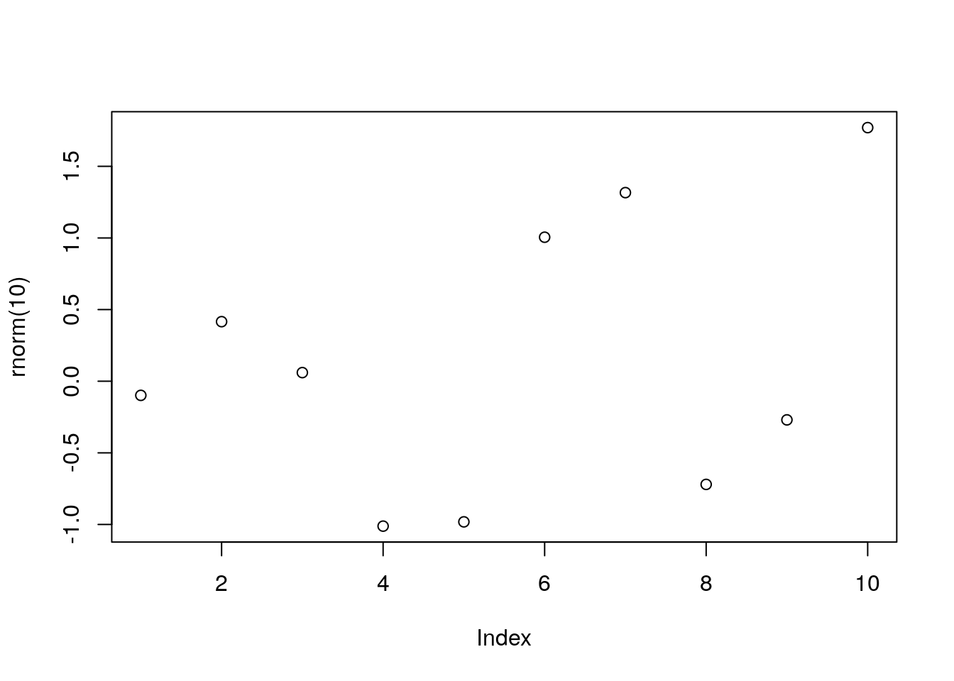
Some useful code chunk options include:
eval=FALSE: to return code only, without output.echo=FALSE: to return output, without code.cache=: to save results so that future compilations are faster.results='hide': to plot figures, without text output.collapse=TRUE: if you want the whole output after the whole code, and not interleaved.warning=FALSE: to supress watning. The same formessage=FALSE, anderror=FALSE.
You can also call r expressions inline.
This is done with a single tick and the r argument.
For instance:
`r rnorm(1)`is a random Gaussian
will output
0.6300902 is a random Gaussian.
13.1.4 BibTex
BibTex is both a file format and a compiler. The bibtex compiler links documents to a reference database stored in the .bib file format.
Bibtex is typically associated with Tex and LaTex typesetting, but it also operates within the markdown pipeline.
Just store your references in a .bib file, add a bibliography: yourFile.bib in the YML preamble of your Rmarkdown file, and call your references from the Rmarkdown text using @referencekey.
Rmarkdow will take care of creating the bibliography, and linking to it from the text.
13.1.5 Compiling
Once you have your .Rmd file written in RMarkdown, knitr will take care of the compilation for you.
You can call the knitr::knitr function directly from some .R file, or more conveniently, use the RStudio (0.96) Knit button above the text editing window.
The location of the output file will be presented in the console.
13.2 bookdown
As previously stated, bookdown is an extension of knitr intended for documents more complicated than simple reports– such as books. Just like knitr, the writing is done in RMarkdown. Being an extension of knitr, bookdown does allow some markdowns that are not supported by other compilers. In particular, it has a more powerful cross referencing system.
13.3 Shiny
Shiny (Chang et al. 2017) is different than the previous systems, because it sets up an interactive web-site, and not a static file. The power of Shiny is that the layout of the web-site, and the settings of the web-server, is made with several simple R commands, with no need for web-programming. Once you have your app up and running, you can setup your own Shiny server on the web, or publish it via Shinyapps.io. The freemium versions of the service can deal with a small amount of traffic. If you expect a lot of traffic, you will probably need the paid versions.
13.3.1 Installation
To setup your first Shiny app, you will need the shiny package. You will probably want RStudio, which facilitates the process.
install.packages('shiny')Once installed, you can run an example app to get the feel of it.
library(shiny)
runExample("01_hello")
Remember to press the Stop button in RStudio to stop the web-server, and get back to RStudio.
13.3.2 The Basics of Shiny
Every Shiny app has two main building blocks.
- A user interface, specified via the
ui.Rfile in the app’s directory. - A server side, specified via the
server.Rfile, in the app’s directory.
You can run the app via the RunApp button in the RStudio interface, of by calling the app’s directory with the shinyApp or runApp functions– the former designed for single-app projects, and the latter, for multiple app projects.
shiny::runApp("my_app") # my_app is the app's directory.The site’s layout, is specified in the ui.R file using one of the layout functions.
For instance, the function sidebarLayout, as the name suggest, will create a sidebar.
More layouts are detailed in the layout guide.
The active elements in the UI, that control your report, are known as widgets.
Each widget will have a unique inputId so that it’s values can be sent from the UI to the server.
More about widgets, in the widget gallery.
The inputId on the UI are mapped to input arguments on the server side.
The value of the mytext inputId can be queried by the server using input$mytext.
These are called reactive values.
The way the server “listens” to the UI, is governed by a set of functions that must wrap the input object.
These are the observe, reactive, and reactive* class of functions.
With observe the server will get triggered when any of the reactive values change.
With observeEvent the server will only be triggered by specified reactive values.
Using observe is easier, and observeEvent is more prudent programming.
A reactive function is a function that gets triggered when a reactive element changes.
It is defined on the server side, and reside within an observe function.
We now analyze the 1_Hello app using these ideas.
Here is the ui.R file.
library(shiny)

shinyUI(fluidPage(

  titlePanel("Hello Shiny!"),

  sidebarLayout(
    sidebarPanel(
      sliderInput(inputId = "bins",
                  label = "Number of bins:",
                  min = 1,
                  max = 50,
                  value = 30)
    ),

    mainPanel(
      plotOutput(outputId = "distPlot")
    )
  )
))
Here is the server.R file:
library(shiny)

shinyServer(function(input, output) {

  output$distPlot <- renderPlot({
    x    <- faithful[, 2]  # Old Faithful Geyser data
    bins <- seq(min(x), max(x), length.out = input$bins + 1)

    hist(x, breaks = bins, col = 'darkgray', border = 'white')
  })
})
Things to note:
ShinyUIis a (deprecated) wrapper for the UI.fluidPageensures that the proportions of the elements adapt to the window side, thus, are fluid.- The building blocks of the layout are a title, and the body. The title is governed by
titlePanel, and the body is governed bysidebarLayout. ThesidebarLayoutincludes thesidebarPanelto control the sidebar, and themainPanelfor the main panel. sliderInputcalls a widget with a slider. ItsinputIdisbins, which is later used by the server within therenderPlotreactive function.plotOutputspecifies that the content of themainPanelis a plot (textOutputfor text). This expectation is satisfied on the server side with therenderPlotfunction (renderText).shinyServeris a (deprecated) wrapper function for the server.- The server runs a function with an
inputand anoutput. The elements ofinputare theinputIds from the UI. The elements of theoutputwill be called by the UI using theiroutputId.
This is the output.
Here is another example, taken from the RStudio Shiny examples.
ui.R:
library(shiny)

fluidPage(

  titlePanel("Tabsets"),

  sidebarLayout(
    sidebarPanel(
      radioButtons(inputId = "dist",
                   label = "Distribution type:",
                   c("Normal" = "norm",
                     "Uniform" = "unif",
                     "Log-normal" = "lnorm",
                     "Exponential" = "exp")),
      br(), # add a break in the HTML page.

      sliderInput(inputId = "n",
                  label = "Number of observations:",
                   value = 500,
                   min = 1,
                   max = 1000)
    ),

    mainPanel(
      tabsetPanel(type = "tabs",
        tabPanel(title = "Plot", plotOutput(outputId = "plot")),
        tabPanel(title = "Summary", verbatimTextOutput(outputId = "summary")),
        tabPanel(title = "Table", tableOutput(outputId = "table"))
      )
    )
  )
)server.R:
library(shiny)

# Define server logic for random distribution application
function(input, output) {

  data <- reactive({
    dist <- switch(input$dist,
                   norm = rnorm,
                   unif = runif,
                   lnorm = rlnorm,
                   exp = rexp,
                   rnorm)

    dist(input$n)
  })

  output$plot <- renderPlot({
    dist <- input$dist
    n <- input$n

    hist(data(), main=paste('r', dist, '(', n, ')', sep=''))
  })

  output$summary <- renderPrint({
    summary(data())
  })

  output$table <- renderTable({
    data.frame(x=data())
  })

}
Things to note:
- We reused the
sidebarLayout. - As the name suggests,
radioButtonsis a widget that produces radio buttons, above thesliderInputwidget. Note the differentinputIds. - Different widgets are separated in
sidebarPanelby commas. br()produces extra vertical spacing (break).tabsetPanelproduces tabs in the main output panel.tabPanelgoverns the content of each panel. Notice the use of various output functions (plotOutput,verbatimTextOutput,tableOutput) with correspondingoutputIds.- In
server.Rwe see the usualfunction(input,output). - The
reactivefunction tells the server the trigger the function wheneverinputchanges. - The
outputobject is constructed outside thereactivefunction. See how the elements ofoutputcorrespond to theoutputIds in the UI.
This is the output:
13.3.3 Beyond the Basics
Now that we have seen the basics, we may consider extensions to the basic report.
13.3.3.1 Widgets
actionButtonAction Button.checkboxGroupInputA group of check boxes.checkboxInputA single check box.dateInputA calendar to aid date selection.dateRangeInputA pair of calendars for selecting a date range.fileInputA file upload control wizard.helpTextHelp text that can be added to an input form.numericInputA field to enter numbers.radioButtonsA set of radio buttons.selectInputA box with choices to select from.sliderInputA slider bar.submitButtonA submit button.textInputA field to enter text.
See examples here.
13.3.3.2 Output Elements
The ui.R output types.
htmlOutputraw HTML.imageOutputimage.plotOutputplot.tableOutputtable.textOutputtext.uiOutputraw HTML.verbatimTextOutputtext.
The corresponding server.R renderers.
renderImageimages (saved as a link to a source file).renderPlotplots.renderPrintany printed output.renderTabledata frame, matrix, other table like structures.renderTextcharacter strings.renderUIa Shiny tag object or HTML.
Your Shiny app can use any R object. The things to remember:
- The working directory of the app is the location of
server.R. - The code before
shinyServeris run only once. - The code inside `
shinyServeris run whenever a reactive is triggered, and may thus slow things.
To keep learning, see the RStudio’s tutorial, and the Biblipgraphic notes herein.
13.3.4 shinydashboard
A template for Shiny to give it s modern look.
13.4 flexdashboard
If you want to quickly write an interactive dashboard, which is simple enough to be a static HTML file and does not need an HTML server, then Shiny may be an overkill. With flexdashboard you can write your dashboard a single .Rmd file, which will generate an interactive dashboard as a static HTML file.
See [http://rmarkdown.rstudio.com/flexdashboard/] for more info.
13.5 Bibliographic Notes
For RMarkdown see here. For everything on knitr see Yihui’s blog, or the book Xie (2015). For a bookdown manual, see Xie (2016). For a Shiny manual, see Chang et al. (2017), the RStudio tutorial, or Hadley’s Book. Video tutorials are available here.
13.6 Practice Yourself
Generate a report using knitr with your name as title, and a scatter plot of two random variables in the body. Save it as PDF, DOCX, and HTML.
Recall that this book is written in bookdown, which is a superset of knitr. Go to the source .Rmd file of the first chapter, and parse it in your head: (https://raw.githubusercontent.com/johnros/Rcourse/master/02-r-basics.Rmd)
References
Chang, Winston, Joe Cheng, JJ Allaire, Yihui Xie, and Jonathan McPherson. 2017. Shiny: Web Application Framework for R. https://CRAN.R-project.org/package=shiny.
Leisch, Friedrich. 2002. “Sweave: Dynamic Generation of Statistical Reports Using Literate Data Analysis.” In Compstat, 575–80. Springer.
Xie, Yihui. 2015. Dynamic Documents with R and Knitr. Vol. 29. CRC Press.
Xie, Yihui. 2016. Bookdown: Authoring Books and Technical Documents with R Markdown. CRC Press.
Recall, S was the original software from which R evolved.↩