Chapter 8 Linear Mixed Models
Sources of variability, i.e. noise, are known in the statistical literature as “random effects”. Specifying these sources determines the correlation structure in our measurements. In the simplest linear models of Chapter 6, we thought of the variability as originating from measurement error, thus independent of anything else. No-correlation, and fixed variability is known as sphericity. Sphericity is of great mathematical convenience, but quite often, unrealistic.
The effects we want to infer on are assumingly non-random, and known “fixed-effects”. Sources of variability in our measurements, known as “random-effects” are usually not the object of interest. A model which has both random-effects, and fixed-effects, is known as a “mixed effects” model. If the model is also linear, it is known as a linear mixed model (LMM). Here are some examples where LMMs arise.
Alternatively, we could consider between-machine variability as another source of uncertainty when inferring on the temporal fixed effect. In which case, would not substract the machine-effect, bur rather, treat it as a random-effect, in the LMM framework.
The unifying theme of the above examples, is that the variability in our data has several sources. Which are the sources of variability that need to concern us? This is a delicate matter which depends on your goals. As a rule of thumb, we will suggest the following view: If information of an effect will be available at the time of prediction, treat it as a fixed effect. If it is not, treat it as a random-effect.
LMMs are so fundamental, that they have earned many names:
Mixed Effects: Because we may have both fixed effects we want to estimate and remove, and random effects which contribute to the variability to infer against.
Variance Components: Because as the examples show, variance has more than a single source (like in the Linear Models of Chapter 6).
Hirarchial Models: Because as Example 8.4 demonstrates, we can think of the sampling as hierarchical– first sample a subject, and then sample its response.
Multilevel Analysis: For the same reasons it is also known as Hierarchical Models.
Repeated Measures: Because we make several measurements from each unit, like in Example 8.4.
Longitudinal Data: Because we follow units over time, like in Example 8.4.
Panel Data: Is the term typically used in econometric for such longitudinal data.
Whether we are aiming to infer on a generative model’s parameters, or to make predictions, there is no “right” nor “wrong” approach. Instead, there is always some implied measure of error, and an algorithm may be good, or bad, with respect to this measure (think of false and true positives, for instance). This is why we care about dependencies in the data: ignoring the dependence structure will probably yield inefficient algorithms. Put differently, if we ignore the statistical dependence in the data we will probably me making more errors than possible/optimal.
We now emphasize:
Like in previous chapters, by “model” we refer to the assumed generative distribution, i.e., the sampling distribution.
In a LMM we specify the dependence structure via the hierarchy in the sampling scheme E.g. caps within machine, students within class, etc. Not all dependency models can be specified in this way! Dependency structures that are not hierarchical include temporal dependencies (AR, ARIMA, ARCH and GARCH), spatial, Markov Chains, and more. To specify dependency structures that are no hierarchical, see Chapter 8 in (the excellent) Weiss (2005).
If you are using LMMs for predictions, and not for inference on the fixed effects or variance components, then see the Supervised Learning Chapter 10. Also recall that machine learning from non-independent observations (such as LMMs) is a delicate matter.
8.1 Problem Setup
We denote an outcome with \(y\) and assume its sampling distribution is given by \[\begin{align} y|x,u = x'\beta + z'u + \varepsilon \tag{8.1} \end{align}\] where \(x\) are the factors with (fixed) effects we want to study, and\(\beta\) denotes these effects. The factors \(z\), with effects \(u\), merely contribute to variability in \(y|x\).
In our repeated measures example (8.2) the treatment is a fixed effect, and the subject is a random effect. In our bottle-caps example (8.3) the time (before vs. after) is a fixed effect, and the machines may be either a fixed or a random effect (depending on the purpose of inference). In our diet example (8.4) the diet is the fixed effect and the subject is a random effect.
Notice that we state \(y|x,z\) merely as a convenient way to do inference on \(y|x\). We could, instead, specify \(Var[y|x]\) directly. The second approach seems less convinient. This is the power of LMMs! We specify the covariance not via the matrix \(Var[z'u|x]\), or \(Var[y|x]\), but rather via the sampling hierarchy.
Given a sample of \(n\) observations \((y_i,x_i,z_i)\) from model (8.1), we will want to estimate \((\beta,u)\). Under some assumption on the distribution of \(\varepsilon\) and \(z\), we can use maximum likelihood (ML). In the context of LMMs, however, ML is typically replaced with restricted maximum likelihood (ReML), because it returns unbiased estimates of \(Var[y|x]\) and ML does not.
8.1.1 Non-Linear Mixed Models
The idea of random-effects can also be extended to non-linear mean models. Formally, this means that \(y|x,z=f(x,z,\varepsilon)\) for some non-linear \(f\). This is known as non-linear-mixed-models, which will not be discussed in this text.
8.1.2 Generalized Linear Mixed Models (GLMM)
You can marry the ideas of random effects, with non-linear link functions, and non-Gaussian distribution of the response. These are known as Generalized Linear Mixed Models (GLMM), which will not be discussed in this text.
8.2 LMMs in R
We will fit LMMs with the lme4::lmer function.
The lme4 is an excellent package, written by the mixed-models Guru Douglas Bates.
We start with a small simulation demonstrating the importance of acknowledging your sources of variability.
Our demonstration consists of fitting a linear model that assumes independence, when data is clearly dependent.
n.groups <- 4 # number of groups
n.repeats <- 2 # samples per group
groups <- rep(1:n.groups, each=n.repeats) %>% as.factor
n <- length(groups)
z0 <- rnorm(n.groups, 0, 10)
(z <- z0[as.numeric(groups)]) # generate and inspect random group effects
## [1] 6.8635182 6.8635182 8.2853917 8.2853917 0.6861244 0.6861244
## [7] -2.4415951 -2.4415951epsilon <- rnorm(n,0,1) # generate measurement error
beta0 <- 2 # this is the actual parameter of interest! The global mean.
y <- beta0 + z + epsilon # sample from an LMMWe can now fit the linear and LMM.
# fit a linear model assuming independence
lm.5 <- lm(y~1)

# fit a mixed-model that deals with the group dependence
library(lme4)
lme.5 <- lmer(y~1|groups)
The summary of the linear model
summary.lm.5 <- summary(lm.5)
summary.lm.5
##
## Call:
## lm(formula = y ~ 1)
##
## Residuals:
## Min 1Q Median 3Q Max
## -6.2932 -3.6148 0.5154 3.9928 5.1632
##
## Coefficients:
## Estimate Std. Error t value Pr(>|t|)
## (Intercept) 5.449 1.671 3.261 0.0138 *
## ---
## Signif. codes: 0 '***' 0.001 '**' 0.01 '*' 0.05 '.' 0.1 ' ' 1
##
## Residual standard error: 4.726 on 7 degrees of freedomThe summary of the LMM
summary.lme.5 <- summary(lme.5)
summary.lme.5
## Linear mixed model fit by REML ['lmerMod']
## Formula: y ~ 1 | groups
##
## REML criterion at convergence: 29.6
##
## Scaled residuals:
## Min 1Q Median 3Q Max
## -1.08588 -0.61820 0.05879 0.53321 1.03325
##
## Random effects:
## Groups Name Variance Std.Dev.
## groups (Intercept) 25.6432 5.0639
## Residual 0.3509 0.5924
## Number of obs: 8, groups: groups, 4
##
## Fixed effects:
## Estimate Std. Error t value
## (Intercept) 5.449 2.541 2.145Look at the standard error of the global mean, i.e., the intercept:
for lm it is 1.671, and for lme it is 2.541.
Why this difference?
Because lm treats the group effect as fixed, while the mixed model treats the group effect as a source of noise/uncertainty.
Inference using lm underestimates our uncertainty in the estimated population mean (\(\beta_0\)).
This is that false-sense of security we may have when ignoring correlations.
8.2.0.1 Relation to Paired t-test
Recall the paired t-test.
Our two-sample–per-group example of the LMM is awfully similar to a pairted t-test.
It would be quite troubeling if the well-known t-test and the oh-so-powerful LMM would lead to diverging conclusions.
In the previous, we inferred on the global mean; a quantity that cancels out when pairing. For a fair comparison, let’s infer on some temporal effect.
Compare the t-statistic below, to the t value in the summary of lme.6.
Luckily, as we demonstrate, the paired t-test and the LMM are equivalent.
So if you follow authors like Barr et al. (2013) that recommend LMMs instead of pairing, remember, these things are sometimes equivalent.
time.fixed.effect <- rep(c('Before','After'), times=4) %>% factor
head(cbind(y,groups,time.fixed.effect))
## y groups time.fixed.effect
## [1,] 9.076626 1 2
## [2,] 8.145687 1 1
## [3,] 10.611710 2 2
## [4,] 10.535547 2 1
## [5,] 2.526772 3 2
## [6,] 3.782050 3 1lme.6 <- lmer(y~time.fixed.effect+(1|groups))
coef(summary(lme.6))## Estimate Std. Error t value
## (Intercept) 5.5544195 2.5513561 2.1770460
## time.fixed.effectBefore -0.2118132 0.4679384 -0.4526518t.test(y~time.fixed.effect, paired=TRUE)$statistic## t
## 0.45265148.2.1 A Single Random Effect
We will use the Dyestuff data from the lme4 package, which encodes the yield, in grams, of a coloring solution (dyestuff), produced in 6 batches using 5 different preparations.
data(Dyestuff, package='lme4')
attach(Dyestuff)
head(Dyestuff)
## Batch Yield
## 1 A 1545
## 2 A 1440
## 3 A 1440
## 4 A 1520
## 5 A 1580
## 6 B 1540And visually
lattice::dotplot(Yield~Batch)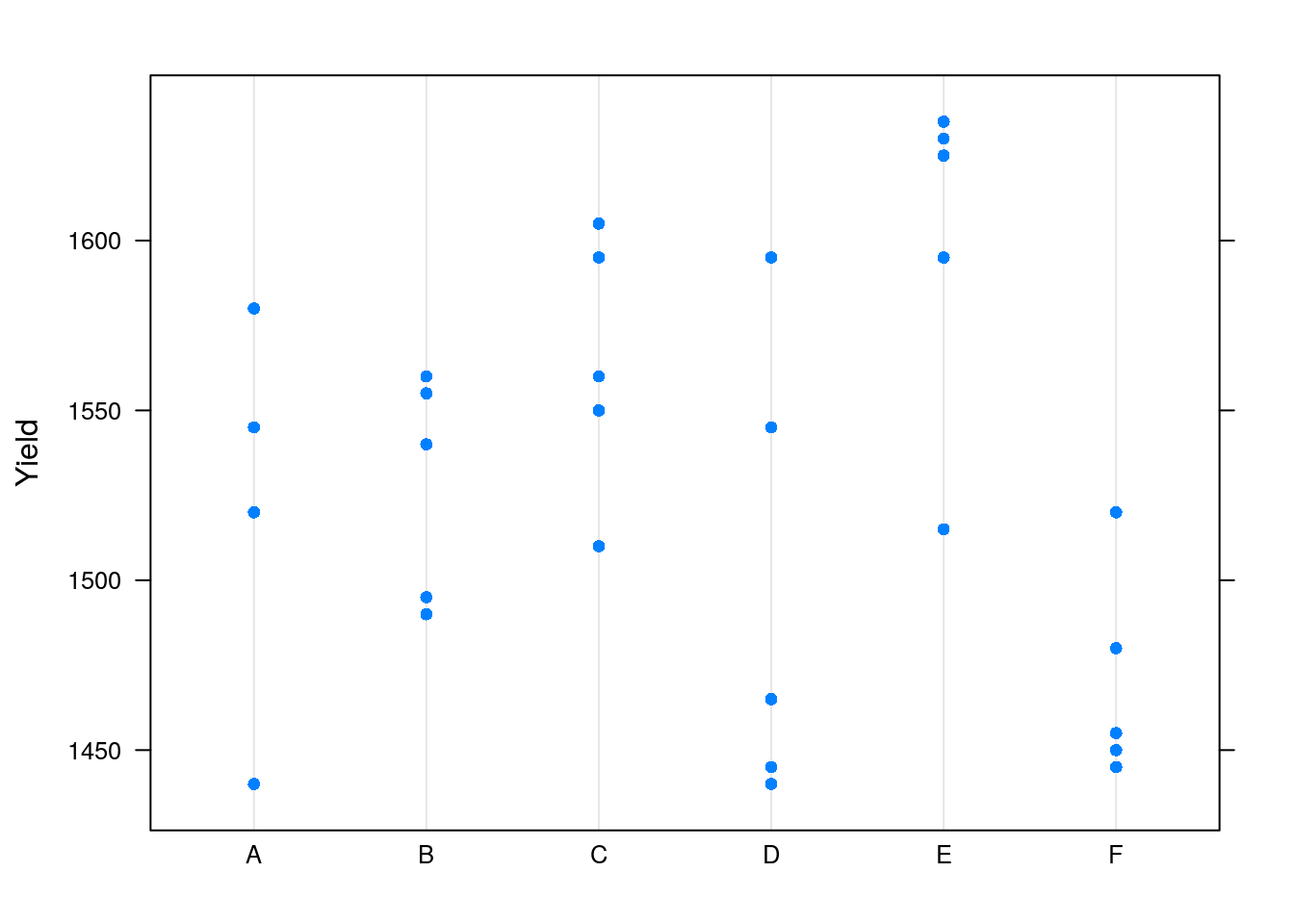
The plot confirms that Yield varies between Batchs.
We do not want to study this batch effect, but we want our inference to apply to new, unseen, batches16.
We thus need to account for the two sources of variability when infering on the (global) mean: the within-batch variability, and the between-batch variability
We thus fit a mixed model, with an intercept and random batch effect.
lme.1<- lmer( Yield ~ 1 + (1|Batch)  , Dyestuff )
summary(lme.1)
## Linear mixed model fit by REML ['lmerMod']
## Formula: Yield ~ 1 + (1 | Batch)
## Data: Dyestuff
##
## REML criterion at convergence: 319.7
##
## Scaled residuals:
## Min 1Q Median 3Q Max
## -1.4117 -0.7634 0.1418 0.7792 1.8296
##
## Random effects:
## Groups Name Variance Std.Dev.
## Batch (Intercept) 1764 42.00
## Residual 2451 49.51
## Number of obs: 30, groups: Batch, 6
##
## Fixed effects:
## Estimate Std. Error t value
## (Intercept) 1527.50 19.38 78.8Things to note:
- The syntax
Yield ~ (1|Batch)tellslme4::lmerto fit a model with a global intercept (1) and a random Batch effect (1|Batch). The|operator is the cornerstone of random effect modelng withlme4::lmer. 1+isn’t really needed.lme4::lmer, likestats::lmadds it be default. We put it there to remind you it is implied.- As usual,
summaryis content aware and has a different behavior forlmeclass objects. - The output distinguishes between random effects (\(u\)), a source of variability, and fixed effect (\(\beta\)), which we want to study. The mean of the random effect is not reported because it is unassumingly 0.
- Were we not interested in standard errors,
lm(Yield ~ Batch)would have returned the same (fixed) effects estimates.
Some utility functions let us query the lme object.
The function coef will work, but will return a cumbersome output. Better use fixef to extract the fixed effects, and ranef to extract the random effects.
The model matrix (of the fixed effects alone), can be extracted with model.matrix, and predictions with predict.
8.2.2 A Full Mixed-Model
In the sleepstudy data, we recorded the reaction times to a series of tests (Reaction), after various subject (Subject) underwent various amounts of sleep deprivation (Day).
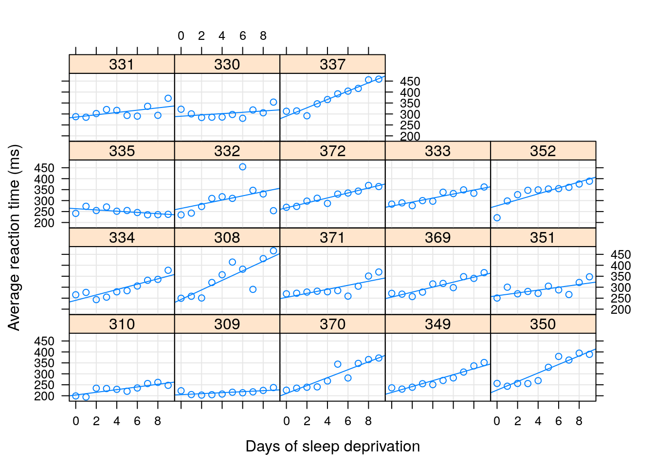
We now want to estimate the (fixed) effect of the days of sleep deprivation on response time, while allowing each subject to have his/hers own effect.
Put differently, we want to estimate a random slope for the effect of day.
The fixed Days effect can be thought of as the average slope over subjects.
lme.3 <- lmer ( Reaction ~ Days + ( Days | Subject ) , data= sleepstudy )Things to note:
~Daysspecifies the fixed effect.- We used the
(Days|Subject)syntax to telllme4::lmerwe want to fit the model~Dayswithin each subject. Just like when modeling withstats::lm,(Days|Subject)is interpreted as(1+Days|Subject), so we get a random intercept and slope, per subject. - Were we not interested in standard erors,
stats::lm(Reaction~Days*Subject)would have returned (alomst) the same effects. Why “almost”? See below…
The fixed day effect is:
fixef(lme.3)## (Intercept) Days
## 251.40510 10.46729The variability in the average response (intercept) and day effect is
ranef(lme.3) %>% lapply(head)## $Subject
## (Intercept) Days
## 308 2.257533 9.1992737
## 309 -40.394272 -8.6205161
## 310 -38.956354 -5.4495796
## 330 23.688870 -4.8141448
## 331 22.258541 -3.0696766
## 332 9.038763 -0.2720535Did we really need the whole lme machinery to fit a within-subject linear regression and then average over subjects?
The short answer is that if we have a enough data for fitting each subject with it’s own lm, we don’t need lme.
The longer answer is that the assumptions on the distribution of random effect, namely, that they are normally distributed, allow us to pool information from one subject to another.
In the words of John Tukey: “we borrow strength over subjects”.
If the normality assumption is true, this is very good news.
If, on the other hand, you have a lot of samples per subject, and you don’t need to “borrow strength” from one subject to another, you can simply fit within-subject linear models without the mixed-models machinery.
This will avoid any assumptions on the distribution of effects over subjects.
For a full discussion of the pro’s and con’s of hirarchial mixed models, consult our Bibliographic Notes.
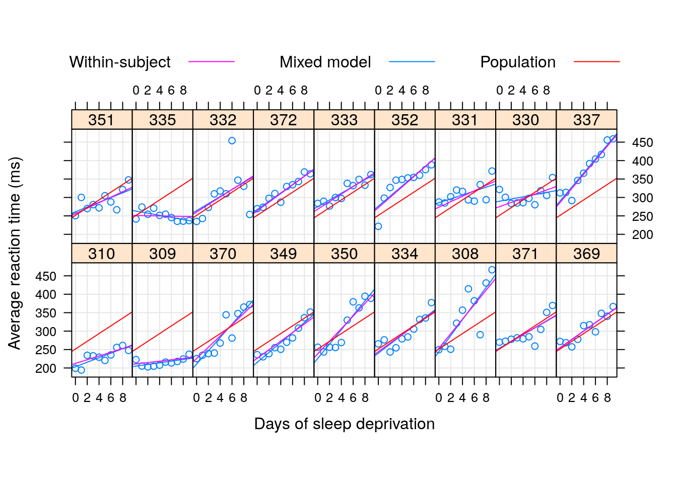
To demonstrate the “strength borrowing”, here is a comparison of the lme, versus the effects of fitting a linear model to each subject separately.
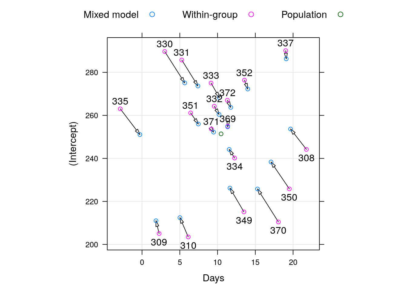
Here is a comparison of the random-day effect from lme versus a subject-wise linear model. They are not the same.
8.2.3 Sparsity and Memory Efficiency
In Chapter 14 we discuss how to efficienty represent matrices in memory. At this point we can already hint that the covariance matrices implied by LMMs are sparse. This fact is exploited in the lme4 package, making it very efficient computationally.
8.3 Serial Correlations in Space/Time
As previously stated, a hierarchical model of the type \(y=x'\beta+z'u+\epsilon\) is a very convenient way to state the correlations of \(y|x\) instead of specifying the matrix \(Var[z'u+\epsilon|x]\) for various \(x\) and \(z\). The hierarchical sampling scheme implies correlations in blocks. What if correlations do not have a block structure? Temporal data or spatial data, for instance, tend to present correlations that decay smoothly in time/space. These correlations cannot be represented via a hirarchial sampling scheme.
One way to go about, is to find a dedicated package for space/time data. For instance, in the Spatio-Temporal Data task view, or the Ecological and Environmental task view.
Instead, we will show how to solve this matter using the nlme package. This is because nlme allows to compond the blocks of covariance of LMMs, with the smoothly decaying covariances of space/time models.
We now use an example from the help of nlme::corAR1.
The nlme::Ovary data is panel data of number of ovarian follicles in different mares (female horse), at various times.
We fit a model with a random Mare effect, and correlations that decay geometrically in time.
In the time-series literature, this is known as an auto-regression of order 1 model, or AR(1), in short.
library(nlme)
head(nlme::Ovary)
## Grouped Data: follicles ~ Time | Mare
## Mare Time follicles
## 1 1 -0.13636360 20
## 2 1 -0.09090910 15
## 3 1 -0.04545455 19
## 4 1 0.00000000 16
## 5 1 0.04545455 13
## 6 1 0.09090910 10fm1Ovar.lme <- nlme::lme(fixed=follicles ~ sin(2*pi*Time) + cos(2*pi*Time),
data = Ovary,
random = pdDiag(~sin(2*pi*Time)),
correlation=corAR1() )
summary(fm1Ovar.lme)## Linear mixed-effects model fit by REML
## Data: Ovary
## AIC BIC logLik
## 1563.448 1589.49 -774.724
##
## Random effects:
## Formula: ~sin(2 * pi * Time) | Mare
## Structure: Diagonal
## (Intercept) sin(2 * pi * Time) Residual
## StdDev: 2.858385 1.257977 3.507053
##
## Correlation Structure: AR(1)
## Formula: ~1 | Mare
## Parameter estimate(s):
## Phi
## 0.5721866
## Fixed effects: follicles ~ sin(2 * pi * Time) + cos(2 * pi * Time)
## Value Std.Error DF t-value p-value
## (Intercept) 12.188089 0.9436602 295 12.915760 0.0000
## sin(2 * pi * Time) -2.985297 0.6055968 295 -4.929513 0.0000
## cos(2 * pi * Time) -0.877762 0.4777821 295 -1.837159 0.0672
## Correlation:
## (Intr) s(*p*T
## sin(2 * pi * Time) 0.000
## cos(2 * pi * Time) -0.123 0.000
##
## Standardized Within-Group Residuals:
## Min Q1 Med Q3 Max
## -2.34910093 -0.58969626 -0.04577893 0.52931186 3.37167486
##
## Number of Observations: 308
## Number of Groups: 11Things to note:
- The fitting is done with the
nlme::lmefunction, and notlme4::lmer. sin(2*pi*Time) + cos(2*pi*Time)is a fixed effect that captures seasonality.- The temporal covariance, is specified using the
correlations=argument. - AR(1) was assumed by calling
correlation=corAR1(). Seenlme::corClassesfor a list of supported correlation structures. - From the summary, we see that a
Marerandom effect has also been added. Where is it specified? It is implied by therandom=argument. Read?lmefor further details.
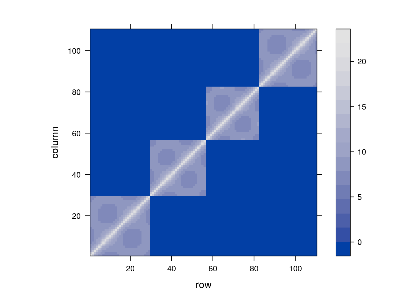
We can now inspect the contrivance implied by our model’s specification.
As expected, we see the blocks of non-null covariance within Mare, but unlike “vanilla” LMMs, the covariance within mare is not fixed. Rather, it decays geometrically with time.
8.4 Extensions
8.4.1 Cluster Robust Standard Errors
As previously stated, random effects are nothing more than a convenient way to specify covariances within a level of a random effect, i.e., within a group/cluster. This is also the motivation underlying cluster robust inference, which is immensely popular with econometricians, but less so elsewhere. With cluster robust inference, we assume a model of type \(y=f(x)+\varepsilon\); unlike LMMs we assume indpenedence (conditonal on \(x\)), but we allow \(\varepsilon\) within clusters defined by \(x\). For a longer comparison between the two approaches, see Michael Clarck’s guide.
8.4.2 Linear Models for Panel Data
nlme and lme4 will probably provide you with all the functionality you need for panel data. If, however, you are trained as an econometrician, and prefer the econometric parlance, then the plm and panelr packages for panel linear models, are just for you. In particular, they allow for cluster-robust covariance estimates, and Durbin–Wu–Hausman test for random effects. The plm package vignette also has an interesting comparison to the nlme package.
8.4.3 Testing Hypotheses on Correlations
After working so hard to model the correlations in observation, we may want to test if it was all required. Douglas Bates, the author of nlme and lme4 wrote a famous cautionary note, found here, on hypothesis testing in mixed models, in particular hypotheses on variance components. Many practitioners, however, did not adopt Doug’s view. Many of the popular tests, particularly the ones in the econometric literature, can be found in the plm package (see Section 6 in the package vignette). These include tests for poolability, Hausman test, tests for serial correlations, tests for cross-sectional dependence, and unit root tests.
8.5 Bibliographic Notes
Most of the examples in this chapter are from the documentation of the lme4 package (Bates et al. 2015). For a general and very applied treatment, see Pinero and Bates (2000). As usual, a hands on view can be found in Venables and Ripley (2013), and also in an excellent blog post by Kristoffer Magnusson For a more theoretical view see Weiss (2005) or Searle, Casella, and McCulloch (2009). Sometimes it is unclear if an effect is random or fixed; on the difference between the two types of inference see the classics: Eisenhart (1947), Kempthorne (1975), and the more recent Rosset and Tibshirani (2018). For an interactive, beatiful visualization of the shrinkage introduced by mixed models, see Michael Clark’s blog. For more on predictions in linear mixed models see Robinson (1991), Rabinowicz and Rosset (2018), and references therein. See Michael Clarck’s guide for various ways of dealing with correlations within groups. For the geo-spatial view and terminology of correlated data, see Christakos (2000), Diggle, Tawn, and Moyeed (1998), Allard (2013), and Cressie and Wikle (2015).
8.6 Practice Yourself
Computing the variance of the sample mean given dependent correlations. How does it depend on the covariance between observations? When is the sample most informative on the population mean?
Think: when is a paired t-test not equivalent to an LMM with two measurements per group?
- Return to the
Penicillindata set. Instead of fitting an LME model, fit an LM model withlm. I.e., treat all random effects as fixed.- Compare the effect estimates.
- Compare the standard errors.
- Compare the predictions of the two models.
- [Very Advanced!] Return to the
Penicillindata and use theglsfunction to fit a generalized linear model, equivalent to the LME model in our text. - Read about the “oats” dataset using
? MASS::oats.Inspect the dependency of the yield (Y) in the Varieties (V) and the Nitrogen treatment (N).- Fit a linear model, does the effect of the treatment significant? The interaction between the Varieties and Nitrogen is significant?
- An expert told you that could be a variance between the different blocks (B) which can bias the analysis. fit a LMM for the data.
- Do you think the blocks should be taken into account as “random effect” or “fixed effect”?
Return to the temporal correlation in Section 8.3, and replace the AR(1) covariance, with an ARMA covariance. Visualize the data’s covariance matrix, and compare the fitted values.
See DataCamps’ Hierarchical and Mixed Effects Models for more self practice.
References
Allard, Denis. 2013. “J.-P. Chiles, P. Delfiner: Geostatistics: Modeling Spatial Uncertainty.” Springer.
Barr, Dale J, Roger Levy, Christoph Scheepers, and Harry J Tily. 2013. “Random Effects Structure for Confirmatory Hypothesis Testing: Keep It Maximal.” Journal of Memory and Language 68 (3). Elsevier: 255–78.
Bates, Douglas, Martin Mächler, Ben Bolker, and Steve Walker. 2015. “Fitting Linear Mixed-Effects Models Using lme4.” Journal of Statistical Software 67 (1): 1–48. https://doi.org/10.18637/jss.v067.i01.
Christakos, George. 2000. Modern Spatiotemporal Geostatistics. Vol. 6. Oxford University Press.
Cressie, Noel, and Christopher K Wikle. 2015. Statistics for Spatio-Temporal Data. John Wiley; Sons.
Diggle, Peter J, JA Tawn, and RA Moyeed. 1998. “Model-Based Geostatistics.” Journal of the Royal Statistical Society: Series C (Applied Statistics) 47 (3). Wiley Online Library: 299–350.
Eisenhart, Churchill. 1947. “The Assumptions Underlying the Analysis of Variance.” Biometrics 3 (1). JSTOR: 1–21.
Kempthorne, Oscar. 1975. “Fixed and Mixed Models in the Analysis of Variance.” Biometrics. JSTOR, 473–86.
Pinero, Jose, and Douglas Bates. 2000. “Mixed-Effects Models in S and S-Plus (Statistics and Computing).” Springer, New York.
Rabinowicz, Assaf, and Saharon Rosset. 2018. “Assessing Prediction Error at Interpolation and Extrapolation Points.” arXiv Preprint arXiv:1802.00996.
Robinson, George K. 1991. “That Blup Is a Good Thing: The Estimation of Random Effects.” Statistical Science. JSTOR, 15–32.
Rosset, Saharon, and Ryan J Tibshirani. 2018. “From Fixed-X to Random-X Regression: Bias-Variance Decompositions, Covariance Penalties, and Prediction Error Estimation.” Journal of the American Statistical Association, nos. just-accepted. Taylor & Francis.
Searle, Shayle R, George Casella, and Charles E McCulloch. 2009. Variance Components. Vol. 391. John Wiley & Sons.
Venables, William N, and Brian D Ripley. 2013. Modern Applied Statistics with S-Plus. Springer Science & Business Media.
Weiss, Robert E. 2005. Modeling Longitudinal Data. Springer Science & Business Media.
Think: why bother treating the
Batcheffect as noise? Should we now just substractBatcheffects? This is not a trick question.↩