Chapter 16 Parallel Computing
You would think that because you have an expensive multicore computer your computations will speed up. Well, unless you actively make sure of that, this will not happen. By default, the operating system will allocate each R session to a single core. You may wonder: why can’t I just write code, and let R (or any other language) figure out what can be parallelised. Sadly, that’s not how things work. It is very hard to design software that can parallelise any algorithm, while adapting to your hardware, operating system, and other the software running on your device. A lot of parallelisation still has to be explicit, but stay tuned for technologies like Ray, Apache Spark, Apache Flink, Chapel, PyTorch, and others, which are making great advances in handling parallelism for you.
To parallelise computationsin with R, we will distinguish between two types of parallelism:
- Parallel R: where the parallelism is managed with R. Discussed in Section 16.3.
- Parallel Extensions: where R calls specialized libraries/routines/software that manage the parallelism themselves. Discussed in Section 16.4.
16.1 When and How to Parallelise?
Your notice computations are too slow, and wonder “why is that?” Should you store your data differently? Should you use different software? Should you buy more RAM? Should you “go cloud”?
Unlike what some vendors will make you think, there is no one-size-fits-all solution to speed problems. Solving a RAM bottleneck may consume more CPU. Solving a CPU bottleneck may consume more RAM. Parallelisation means using multiple CPUs simultaneously. It will thus aid with CPU bottlenecks, but may consume more RAM. Parallelising is thus ill advised when dealing with a RAM bottleneck. Memory bottlenecks are released with efficient memory representations or out-of-memory algorithms (Chapters 14 and 15).
When deciding if, and how, to parallelise, it is crucial that you diagnose your bottleneck. The good news is- that diagnostics is not too hard. Here are a few pointers:
You never drive without looking at your dashboard; you should never program without looking at your system monitors. Windows users have their Task Manager; Linux users have top, or preferably, htop; Mac users have the Activity Monitor. The system monitor will inform you how your RAM and CPUs are being used.
If you forcefully terminate your computation, and R takes a long time to respond, you are probably dealing with a RAM bottleneck.
Profile your code to detect how much RAM and CPU are consumed by each line of code. See Hadley’s guide.
In the best possible scenario, the number of operations you can perform scales with the number of processors: \[time * processors = operations\]. This is called perfect scaling. It is rarely observed in practice, since parallelising incurs some computational overhead: setting up environments, copying memory, … For this reason, the typical speedup is sub-linear. Computer scientists call this Amdahl’s law; remember it.
16.2 Terminology
Here are some terms we will be needing.
16.2.1 Hardware:
- Cluster: A collection of interconnected computers.
- Node/Machine: A single physical machine in the cluster. Components of a single node do not communicate via the cluster’s network, but rather, via the node’s circuitry.
- Processor/Socket/CPU/Core: The physical device in a computer that make computations. A modern laptop will have about 4-8 cores. A modern server may have hundreds of cores.
- RAM: Random Access Memory. One of many types of memory in a computer. Possibly the most relevant type of memory when computing with data.
- GPU: Graphical Processing Unit. A computing unit, separate from the CPU. Originally dedicated to graphics and gaming, thus its name. Currently, GPUs are extremely popular for fitting and servicing Deep Neural Networks.
- TPU: Tensor Processing Unit. A computing unit, dedicated to servicing and fitting Deep Neural Networks.
16.2.2 Software:
- Process: A sequence of instructions in memory, with accompanying data. Various processes typically see different locations of memory. Interpreted languages like R, and Python operate on processes.
- Thread: A sub-sequence of instructions, within a process. Various threads in a process may see the same memory. Compiled languages like C, C++, may operate on threads.
16.3 Parallel R
R provides many frameworks to parallelise execution.
The operating system allocates each R session to a single process.
Any parallelisation framework will include the means for starting R processes, and the means for communicating between these processes.
Except for developers, a typical user will probably use some high-level R package which will abstract away these stages.
16.3.1 Starting a New R Processes
A R process may strat a new R process in various ways. The new process may be called a child process, a slave process, and many other names. Here are some mechanisms to start new processes.
Fork: Imagine the operating system making a copy of the currently running R process. The fork mechanism, unique to Unix and Linux, clones a process with its accompanying instructions and data. All forked processes see the same memory in read-only mode. Copies of the data are made when the process needs to change the data.
System calls: Imagine R as a human user, that starts a new R session. This is not a forked porcess. The new process, called spawn process cannot access the data and instructions of the parent process.
16.3.2 Inter-process Communication
Now that you have various R processes running, how do they communicate?
Socket: imagine each R process as a standalone computer in the network. Data can be sent via a network interface. Unlike PVM, MPI and other standards, information sent does not need to be format in any particular way, provided that the reciever knows how it is formatted. This is not a problem when sending from R to R.
Parallel Virtual Machine (PVM): a communication protocol and software, developed the University of Tennessee, Oak Ridge National Laboratory and Emory University, and first released in 1989. Runs on Windows and Unix, thus allowing to compute on clusters running these two operating systems. Noways, it is mostly replaced by MPI. The same group responsible for PVM will later deliver pbdR 16.3.6.
Message Passing Interface (MPI): A communication protocol that has become the de-facto standard for communication in large distributed clusters. Particularly, for heterogeneous computing clusters with varying operating systems and hardware. The protocol has various software implementations such as OpenMPI and MPICH, Deino, LAM/MPI. Interestingly, large computing clusters use MPI, while modern BigData analysis platforms such as Spark, and Ray do not. Why is this? See Jonathan Dursi’s excellent blog post.
NetWorkSpaces (NWS): A master-slave communication protocol where the master is not an R-session, but rather, an NWS server.
For more on inter-process communication, see Wiki.
16.3.3 The parallel Package
The parallel package, maintained by the R-core team, was introduced in 2011 to unify two popular parallisation packages: snow and multicore. The multicore package was designed to parallelise using the fork mechanism, on Linux machines. The snow package was designed to parallelise Socket, PVM, MPI, and NWS mechanisms. R processes started with snow are not forked, so they will not see the parent’s data. Data will have to be copied to child processes. The good news: snow can start R processes on Windows machines, or remotely machines in the cluster.
TOOD: add example.
16.3.4 The foreach Package
For reasons detailed in Kane et al. (2013), we recommend the foreach parallelisation package (Analytics and Weston 2015). It allows us to:
Decouple between the parallel algorithm and the parallelisation mechanism: we write parallelisable code once, and can later switch between parallelisation mechanisms. Currently supported mechanisms include:
- fork: Called with the doMC backend.
- MPI, VPM, NWS: Called with the doSNOW or doMPI backends.
- futures: Called with the doFuture backend.
- redis: Called with the doRedis backend. Similar to NWS, only that data made available to different processes using Redis.
- Future mechanism may also be supported.
Combine with the
big.matrixobject from Chapter 15 for shared memory parallelisation: all the machines may see the same data, so that we don’t need to export objects from machine to machine.
Let’s start with a simple example, taken from “Getting Started with doParallel and foreach”.
library(doParallel)
cl <- makeCluster(2, type = 'SOCK')
registerDoParallel(cl)
result <- foreach(i=1:3) %dopar% sqrt(i)
class(result)
## [1] "list"result## [[1]]
## [1] 1
##
## [[2]]
## [1] 1.414214
##
## [[3]]
## [1] 1.732051Things to note:
makeClustercreates an object with the information our cluster. On a single machine it is very simple. On a cluster of machines, you will need to specify the IP addresses, or other identifier, of the machines.registerDoParallelis used to inform the foreach package of the presence of our cluster.- The
foreachfunction handles the looping. In particular note the%dopar%operator that ensures that looping is in parallel.%dopar%can be replaced by%do%if you want serial looping (like theforloop), for instance, for debugging. - The output of the various machines is collected by
foreachto a list object. - In this simple example, no data is shared between machines so we are not putting the shared memory capabilities to the test.
- We can check how many workers were involved using the
getDoParWorkers()function. - We can check the parallelisation mechanism used with the
getDoParName()function.
Here is a more involved example. We now try to make Bootstrap inference on the coefficients of a logistic regression. Bootstrapping means that in each iteration, we resample the data, and refit the model.
x <- iris[which(iris[,5] != "setosa"), c(1,5)]
trials <- 1e4
r <- foreach(icount(trials), .combine=cbind) %dopar% {
  ind <- sample(100, 100, replace=TRUE)
  result1 <- glm(x[ind,2]~x[ind,1], family=binomial(logit))
  coefficients(result1)
}
Things to note:
- As usual, we use the
foreachfunction with the%dopar%operator to loop in parallel. - The
iterators::icountfunction generates a counter that iterates over its argument. - The object
xis magically avaiable at all child processes, even though we did not fork R. This is thanks toforachwhich guesses what data to pass to children. - The
.combine=cbindargument tells theforeachfunction how to combine the output of different machines, so that the returned object is not the default list. - To run a serial version, say for debugging, you only need to replace
%dopar%with%do%.
 r <- foreach(icount(trials), .combine=cbind) %do% {
 ind <- sample(100, 100, replace=TRUE)
 result1 <- glm(x[ind,2]~x[ind,1], family=binomial(logit))
 coefficients(result1)
 }
Let’s see how we can combine the power of bigmemory and foreach by creating a file mapped big.matrix object, which is shared by all machines.
The following example is taken from Kane et al. (2013), and uses the big.matrix object we created in Chapter 15.
library(bigmemory)
x <- attach.big.matrix("airline.desc")

library(foreach)
library(doSNOW)
cl <- makeSOCKcluster(names=rep("localhost", 4)) # make a cluster of 4 machines
registerDoSNOW(cl) # register machines for foreach()
xdesc <- describe(x)

G <- split(1:nrow(x), x[, "BENE_AGE_CAT_CD"]) # Split the data along `BENE_AGE_CAT_CD`.

GetDepQuantiles <- function(rows, data) {
 quantile(data[rows, "CAR_LINE_ICD9_DGNS_CD"],
          probs = c(0.5, 0.9, 0.99),
          na.rm = TRUE)
} # Function to extract quantiles

qs <- foreach(g = G, .combine = rbind) %dopar% {
 library("bigmemory")
 x <- attach.big.matrix(xdesc)
 GetDepQuantiles(rows = g, data = x)
} # get quantiles, in parallel
qs
## 50% 90% 99%
## result.1 558 793 996
## result.2 518 789 996
## result.3 514 789 996
## result.4 511 789 996
## result.5 511 790 996
## result.6 518 796 995Things to note:
bigmemory::attach.big.matrixcreates an R big.matrix object from a matrix already existing on disk. See Section 15.3.1 for details.snow::makeSOCKclustercreates cluster of R processes communicating via sockets.bigmemory::describerecovres a pointer to the big.matrix object, that will be used to call it from various child proceeses.- Because R processes were not forked, each child need to load the bigmemory package separately.
Can only big.matrix objects be used to share data between child processes? No. There are many mechanism to share data. We use big.matrix merely for demonstration.
16.3.4.1 Fork or Socket?
On Linux and Unix machines you can use both the fork mechanism of the multicore package, and the socket mechanism of the snow package. Which is preferable? Fork, if available. Here is a quick comparison.
library(nycflights13)
flights$ind <- sample(1:10, size = nrow(flights), replace = TRUE) #split data to 10.

timer <- function(i) max(flights[flights$ind==i,"distance"]) # an arbitrary function

library(doMC)
registerDoMC(cores = 10) # make a fork cluster
system.time(foreach (i=1:10, .combine = 'c') %dopar% timer(i)) # time the fork cluster
## user system elapsed
## 0.013 0.409 0.429library(parallel)
library(doParallel)
cl <- makeCluster(10, type="SOCK") # make a socket cluster.
registerDoParallel(cl)
system.time(foreach (i=1:10, .combine = 'c') %dopar% timer(i)) # time the socket cluster## user system elapsed
## 1.054 0.161 2.020stopCluster(cl) # close the clusterThings to note:
doMC::registerDoMCwas used to stard and register the forked cluster.parallel::makeClusterwas used to stard the socket cluster. It was registered withdoParallel::registerDoParallel.- After registering the cluster, the foreach code is exactly the same.
- The clear victor is fork: sessions start faster, and computations finish faster. Sadly, we recall that forking is impossible on Windows machines, or in clusters that consist of several machines.
- We did not need to pass
flightsto the different workers.foreach::foreachtook care of that for us.
For fun, let’s try the same with data.table.
library(data.table)
flights.DT <- as.data.table(flights)
system.time(flights.DT[,max(distance),ind])
## user system elapsed
## 0.058 0.080 0.103No surprises there.
If you can store your data in RAM, data.table is still the fastest.
16.3.5 Rdsm
TODO
16.3.6 pbdR
TODO
16.4 Parallel Extensions
As we have seen, R can be used to write explicit parallel algorithms. Some algorithms, however, are so basic that others have already written and published their parallel versions. We call these parallel extensions. Linear algebra, and various machine learning algorithms are examples we now discuss.
16.4.1 Parallel Linear Algebra
R ships with its own linear algebra algorithms, known as Basic Linear Algebra Subprograms: BLAS. To learn the history of linear algebra in R, read Maechler and Bates (2006). For more details, see our Bibliographic notes. BLAS will use a single core, even if your machines has many more. There are many linear algebra libraries out there, and you don’t need to be a programmer to replace R’s BLAS. Cutting edge linear algebra libraries such as OpenBLAS, Plasma, and Intel’s MKL, will do your linear algebra while exploiting the many cores of your machine. This is very useful, since all machines today have multiple cores, and linear algebra is at the heart of all statistics and machine learning.
Installing these libraries requires some knowldge in system administration. It is fairly simple under Ubuntu and Debian linux, and may be more comlicated on other operating systems. Installing these is outside the scope of this text. We will thus content ourselves with the following pointers:
- Users can easily replace the BLAS libraries shipped with R, with other libraries such as OpenBLAS, and MKL. These will parallelise linear algebra for you.
- Installation is easier for Ubuntu and Debian Linux, but possible in all systems.
- For specific tasks, such as machine learning, you may not need an all-pupose paralle linear algebra library. If you want machine learning in parallel, there are more specialized libraries. In the followig, we demonstrate Spark (16.4.3), and H2O (16.4.4).
- Read our word of caution on nested parallelism (16.5) if you use parallel linear algebra within child R processes.
16.4.2 Parallel Data Munging with data.table
We have discussed data.table in Chapter 4.
We now recall it to emphasize that various operations in data.table are done in parallel, using OpenMP.
For instance, file imports can done in paralle: each thread is responsible to impot a subset of the file.
First, we check how many threads data.table is setup to use?
library(data.table)
getDTthreads(verbose=TRUE)
## omp_get_num_procs()==8
## R_DATATABLE_NUM_PROCS_PERCENT=="" (default 50)
## R_DATATABLE_NUM_THREADS==""
## omp_get_thread_limit()==2147483647
## omp_get_max_threads()==1
## OMP_THREAD_LIMIT==""
## OMP_NUM_THREADS==""
## data.table is using 4 threads. This is set on startup, and by setDTthreads(). See ?setDTthreads.
## RestoreAfterFork==true## [1] 4Things to note:
data.table::getDTthreadsto get some info on my machine, and curentdata.tablesetup. Use theverbose=TRUEflag for extra details.- omp_get_max_threads informs me how many threads are available in my machine.
- My current
data.tableconfiguraton is in the last line of the output.
We then import with data.table::fread and inspect CPU usage with the top linux command.
air <- fread('data/2010_BSA_Carrier_PUF.csv')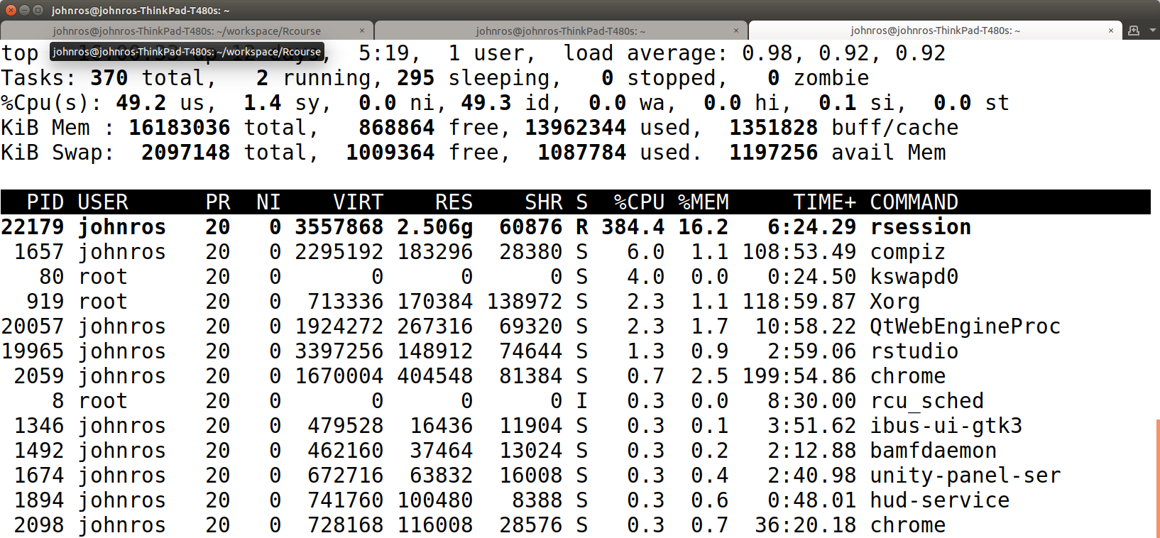
The CPU usage of fread() is 384.4%. This is because data.table is setup to use 4 threads simultanously.
data.table is that it will not parallelize when called from a forked process.
This behaviour will avoid the nested parallelism we cautioned from in 16.5.
After doing parallel imports, let’s try parallel aggregation.
n <-  5e6
N <- n
k <-  1e4

setDTthreads(threads = 0) # use all available cores
getDTthreads() # print available threads
## [1] 8DT <- data.table(x = rep_len(runif(n), N),
y = rep_len(runif(n), N),
grp = rep_len(sample(1:k, n, TRUE), N))
system.time(DT[, .(a = 1L), by = "grp"])## user system elapsed
## 0.416 0.020 0.073setDTthreads(threads = 1) # use a single thread
system.time(DT[, .(a = 1L), by = "grp"])## user system elapsed
## 0.147 0.000 0.146Things to note:
- Parallel aggregation is indeed much faster.
- Cores scaled by 8 fold. Time scaled by less. The scaling is not perfect. Remember Amdahl’s law.
- This example was cooked to emphasize the difference. You may not enjoy such speedups in all problems.
If the data does not fit in our RAM, we cannot enjoy data.tables.
If the data is so large that it does not fit into RAM29, nor into your local disk, you will need to store, and compute with it, in a distributed cluster.
In the next section, we present a very popular system for storing, munging, and learning, with massive datasets.
16.4.3 Spark
Spark is the brainchild of Matei Zaharia, in 2009, as part of his PhD studies at University of California, Berkeley ’s AMPLab. To understand Spark we need some background.
The software that manages files on your disk is the file system. On personal computers, you may have seen names like FAT32, NTFS, EXT3, or others. Those are file systems for disks. If your data is too big to be stored on a single disk, you may distribute it on several machines. When doing so, you will need a file systems that is designed for distributed clusters. A good cluster file system, is crucial for the performance of your cluster. Part of Google strength is in its powerful file system, the Google File System. If you are not at Google, you will not have access to this file system. Luckily, there are many other alternatives. The Hadoop File System, HDFS, that started at Yahoo, later donated to the Apache Foundation, is a popular alternative. With the HDFS you can store files in a cluster.
For doing statistics, you need software that is compatible with the file system. This is true for all file systems, and in particular, HDFS. A popular software suit that was designed to work with HDFS is Hadoop. Alas, Hadoop was not designed for machine learning. Hadoop for reasons of fault tolerance, Hadoop stores its data disk. Machine learning consists of a lot iterative algorithms that requires fast and repeated data reads. This is very slow if done from the disk. This is where Spark comes in. Spark is a data oriented computing environment over distributed file systems. Let’s parse that:
- “data oriented”: designed for statistics and machine learning, which require a lot of data, that is mostly read and not written.
- “computing environment”: it less general than a full blown programming language, but it allows you to extend it.
- “over distributed file systems”: it ingests data that is stored in distributed clusters, managed by HDFS or other distributed file system.
Let’s start a Spark server on our local machine to get a feeling of it. We will not run from a cluster, so that you may experiment with it yourself.
library(sparklyr)
spark_install(version = "2.4.0") # will download Spark on first run.
sc <- spark_connect(master = "local")
Things to note:
spark_installwill download and install Spark on your first run. Make sure to update the version number, since my text may be outdated by the time you read it.- I used the sparklyr package from RStudio. There is an alternative package from Apache: SparkR.
spark_connectopens a connection to the (local) Spark server. When working in a cluster, with many machines, themaster=argumnt infrorms R which machine is the master, a.k.a. the “driver node”. Consult your cluster’s documentation for connection details.- After running
spark_connect, the connection to the Sprak server will appear in RStudio’s Connection pane.
Let’s load and aggregate some data:
library(nycflights13)
flights_tbl<- copy_to(dest=sc, df=flights, name='flights', overwrite = TRUE)
class(flights_tbl)
## [1] "tbl_spark" "tbl_sql" "tbl_lazy" "tbl"library(dplyr)
system.time(delay<-flights_tbl %>%
group_by(tailnum) %>%
summarise(
count=n(),
dist=mean(distance, na.rm=TRUE),
delay=mean(arr_delay, na.rm=TRUE)) %>%
filter(count>20, dist<2000, !is.na(delay)) %>%
collect())## user system elapsed
## 0.216 0.587 1.699delay## # A tibble: 2,961 x 4
## tailnum count dist delay
## <chr> <dbl> <dbl> <dbl>
## 1 N24211 130 1330. 7.7
## 2 N793JB 283 1529. 4.72
## 3 N657JB 285 1286. 5.03
## 4 N633AA 24 1587. -0.625
## 5 N9EAMQ 248 675. 9.24
## 6 N3GKAA 77 1247. 4.97
## 7 N997DL 63 868. 4.90
## 8 N318NB 202 814. -1.12
## 9 N651JB 261 1408. 7.58
## 10 N841UA 96 1208. 2.10
## # … with 2,951 more rowsThings to note:
copy_toexports from R to Sprak. Typically, my data will already be waiting in Sprak, since the whole motivation is that it does not fit on my disk.- Notice the
collectcommand at the end. As the name suggests, this will collect results from the various worker/slave machines. - I have used the dplyr syntax and not my favorite data.table syntax. This is because sparklyr currently supports the splyr syntax, or plain SQL with the DBI package.
To make the most of it, you will porbably be running Spark on some cluster.
You should thus consult your cluster’s documentation in order to connect to it.
In our particular case, the data is not very big so it fits into RAM.
We can thus compare performance to data.table, only to re-discover, than if data fits in RAM, there is no beating data.table.
library(data.table)
flight.DT <- data.table(flights)
system.time(flight.DT[,.(distance=mean(distance),delay=mean(arr_delay),count=.N),by=tailnum][count>20 & distance<2000 & !is.na(delay)])
## user system elapsed
## 0.031 0.000 0.031Let’s disconnect from the Spark server.
spark_disconnect(sc)## NULLSpark comes with a set of learning algorithms called MLLib. Consult the online documentation to see which are currently available. If your data is happily stored in a distributed Spark cluster, and the algorithm you want to run is not available, you have too options: (1) use extensions or (2) write your own.
Writing your own algorithm and dispatching it to Spark can be done a-la apply style with sparklyr::spark_apply. This, however, would typically be extremely inneficient. You are better off finding a Spark extension that does what you need.
See the sparklyr CRAN page, and in particular the Reverse Depends section, to see which extensions are available.
One particular extension is rsparkling, which allows you to apply H2O’s massive library of learning algorithms, on data stored in Spark.
We start by presenting H2O.
16.4.4 H2O
H2O can be thought of as a library of efficient distributed learning algorithm, that run in-memory, where memory considerations and parallelisation have been taken care of for you.
Another way to think of it is as a “machine learning service”.
For a (massive) list of learning algorithms implemented in H2O, see their documentaion.
H2O can run as a standalone server, or on top of Spark, so that it may use the Spark data frames.
We start by working with H2O using H2O’s own data structures, using h2o package.
We later discuss how to use H2O using Spark’s data structures (16.4.4.1).
#install.packages("h2o")
library(h2o)

h2o.init(nthreads=2)
## Connection successful!
##
## R is connected to the H2O cluster:
## H2O cluster uptime: 1 minutes 38 seconds
## H2O cluster timezone: Etc/UTC
## H2O data parsing timezone: UTC
## H2O cluster version: 3.26.0.2
## H2O cluster version age: 2 months and 13 days
## H2O cluster name: H2O_started_from_R_rstudio_kxj197
## H2O cluster total nodes: 1
## H2O cluster total memory: 3.42 GB
## H2O cluster total cores: 8
## H2O cluster allowed cores: 8
## H2O cluster healthy: TRUE
## H2O Connection ip: localhost
## H2O Connection port: 54321
## H2O Connection proxy: NA
## H2O Internal Security: FALSE
## H2O API Extensions: Amazon S3, XGBoost, Algos, AutoML, Core V3, Core V4
## R Version: R version 3.6.1 (2019-07-05)Things to note:
- We did not install the H2O server;
install.packages("h2o")did it for us. h2o.initfires the H2O server. Usenthreadsto manually control the number of threads, or use the defaults. “H2O cluster total cores” informs you of the number of potential cores. “H2O cluster allowed cores” was set bynthreads, and informs of the number of actual cores that will be used.- Read
?h2o.initfor the (massive) list of configuration parameters available.
h2o.no_progress() # to supress progress bars.
data("spam", package = 'ElemStatLearn')
spam.h2o <- as.h2o(spam, destination_frame = "spam.hex") # load to the H2O server
h2o.ls() # check avaialbe data in the server
## key
## 1 RTMP_sid_a49b_4
## 2 RTMP_sid_a49b_6
## 3 modelmetrics_our.rf@-7135746841792491802_on_RTMP_sid_a49b_4@1783194943144526592
## 4 our.rf
## 5 predictions_8b59_our.rf_on_RTMP_sid_a49b_6
## 6 spam.hexh2o.describe(spam.h2o) %>% head # the H2O version of summary()## Label Type Missing Zeros PosInf NegInf Min Max Mean Sigma
## 1 A.1 real 0 3548 0 0 0 4.54 0.10455336 0.3053576
## 2 A.2 real 0 3703 0 0 0 14.28 0.21301456 1.2905752
## 3 A.3 real 0 2713 0 0 0 5.10 0.28065638 0.5041429
## 4 A.4 real 0 4554 0 0 0 42.81 0.06542491 1.3951514
## 5 A.5 real 0 2853 0 0 0 10.00 0.31222343 0.6725128
## 6 A.6 real 0 3602 0 0 0 5.88 0.09590089 0.2738241
## Cardinality
## 1 NA
## 2 NA
## 3 NA
## 4 NA
## 5 NA
## 6 NAh2o.table(spam.h2o$spam)## spam Count
## 1 email 2788
## 2 spam 1813
##
## [2 rows x 2 columns]# Split to train and test
splits <- h2o.splitFrame(data = spam.h2o, ratios = c(0.8))
train <- splits[[1]]
test <- splits[[2]]
# Fit a random forest
rf <- h2o.randomForest(
x = names(spam.h2o)[-58],
y = c("spam"),
training_frame = train,
model_id = "our.rf")
# Predict on test set
predictions <- h2o.predict(rf, test)
head(predictions)## predict email spam
## 1 spam 0.040000000 0.9600000
## 2 spam 0.003636364 0.9963636
## 3 email 0.647725372 0.3522746
## 4 spam 0.200811689 0.7991883
## 5 spam 0.000000000 1.0000000
## 6 spam 0.213333334 0.7866667Things to note:
- H2O objects behave a lot like data.frame/tables.
- To compute on H2O objects, you need dedicated function. They typically start with “h2o” such as
h2o.table, andh2o.randomForest. h2o.randomForest, and other H2O functions, have their own syntax with many many options. Make sure to read?h2o.randomForest.
16.4.4.1 Sparkling-Water
The h2o package (16.4.4) works with H2OFrame class objects.
If your data is stored in Spark, it may be more natural to work with Spark DataFrames instead of H2OFrames.
This is exactly the purpose of the Sparkling-Water system.
R users can connect to it using the RSparkling package, written and maintained by H2O.
16.5 Caution: Nested Parallelism
A common problem when parallelising is that the processes you invoke explicitely, may themselves invoke other processes.
Consider a user forking multiple processes, each process calling data.table, which itself will invoke multiple threads.
This is called nested parallelism, and may cause you to lose control of the number of machine being invoked.
The operating system will spend most of its time with housekeeping, instead of doing your computations.
Luckily, data.table was designed to avoid this.
If you are parallelising your linear algebra with OpenBLAS, you may control nested parallelism with the package RhpcBLASctl. In other cases, you should be aware of this, and may need to consult an expert.
16.6 Bibliographic Notes
To understand how computers work in general, see Bryant and O’Hallaron (2015). For a brief and excellent explanation on parallel computing in R see Schmidberger et al. (2009). For a full review see Chapple et al. (2016). For a blog-level introduction see ParallelR. For an up-to-date list of packages supporting parallel programming see the High Performance Computing R task view. For some theory of distributed machine learning, see J. D. Rosenblatt and Nadler (2016).
An excellent video explaining data.table and H2O, by the author of `data.table, is this.
More benchmarks in here.
More on Spark with R in Mastering Apache Spark with R.
For a blog level introduction to linear algebra in R see Joseph Rickert’s entry. For a detailed discussion see Oancea, Andrei, and Dragoescu (2015).
References
Analytics, Revolution, and Steve Weston. 2015. Foreach: Provides Foreach Looping Construct for R. https://CRAN.R-project.org/package=foreach.
Bryant, Randal E, and David R O’Hallaron. 2015. Computer Systems: A Programmer’s Perspective Plus Masteringengineering with Pearson eText–Access Card Package. Pearson.
Chapple, Simon R, Eilidh Troup, Thorsten Forster, and Terence Sloan. 2016. Mastering Parallel Programming with R. Packt Publishing Ltd.
Kane, Michael J, John Emerson, Stephen Weston, and others. 2013. “Scalable Strategies for Computing with Massive Data.” Journal of Statistical Software 55 (14): 1–19.
Maechler, Martin, and Douglas Bates. 2006. “2nd Introduction to the Matrix Package.” R Core Development Team. Accessed on: Https://Stat. Ethz. Ch/R-Manual/R-Devel/Library/Matrix/Doc/Intro2Matrix. Pdf.
Oancea, Bogdan, Tudorel Andrei, and Raluca Mariana Dragoescu. 2015. “Accelerating R with High Performance Linear Algebra Libraries.” arXiv Preprint arXiv:1508.00688.
Rosenblatt, Jonathan D, and Boaz Nadler. 2016. “On the Optimality of Averaging in Distributed Statistical Learning.” Information and Inference: A Journal of the IMA 5 (4). Oxford University Press: 379–404.
Schmidberger, Markus, Martin Morgan, Dirk Eddelbuettel, Hao Yu, Luke Tierney, and Ulrich Mansmann. 2009. “State of the Art in Parallel Computing with R.” Journal of Statistical Software 47 (1).
Recall that you can buy servers wth 1TB of RAM and more. So we are talking about A LOT of data!↩